Fortuna Trend Predictor**Fortuna Trend Predictor**
### Overview
**Fortuna Trend Predictor** is a powerful trend analysis tool that combines multiple technical indicators to estimate trend strength, volatility, and probability of price movement direction. This indicator is designed to help traders identify potential trend shifts and confirm trade setups with improved accuracy.
### Key Features
- **Trend Strength Analysis**: Uses the difference between short-term and long-term Exponential Moving Averages (EMA) normalized by the Average True Range (ATR) to determine trend strength.
- **Directional Strength via ADX**: Calculates the Average Directional Index (ADX) manually to measure the strength of the trend, regardless of its direction.
- **Probability Estimation**: Provides a probabilistic assessment of price movement direction based on trend strength.
- **Volume Confirmation**: Incorporates a volume filter that validates signals when the trading volume is above its moving average.
- **Volatility Filter**: Uses ATR to identify high-volatility conditions, helping traders avoid false signals during low-volatility periods.
- **Overbought & Oversold Levels**: Includes RSI-based horizontal reference lines to highlight potential reversal zones.
### Indicator Components
1. **ATR (Average True Range)**: Measures market volatility and serves as a denominator to normalize EMA differences.
2. **EMA (Exponential Moving Averages)**:
- **Short EMA (20-period)** - Captures short-term price movements.
- **Long EMA (50-period)** - Identifies the overall trend.
3. **Trend Strength Calculation**:
- Formula: `(Short EMA - Long EMA) / ATR`
- The higher the value, the stronger the trend.
4. **ADX Calculation**:
- Computes +DI and -DI manually to generate ADX values.
- Higher ADX indicates a stronger trend.
5. **Volume Filter**:
- Compares current volume to a 20-period moving average.
- Signals are more reliable when volume exceeds its average.
6. **Volatility Filter**:
- Detects whether ATR is above its own moving average, multiplied by a user-defined threshold.
7. **Probability Plot**:
- Formula: `50 + 50 * (Trend Strength / (1 + abs(Trend Strength)))`
- Values range from 0 to 100, indicating potential movement direction.
### How to Use
- When **Probability Line is above 70**, the trend is strong and likely to continue.
- When **Probability Line is below 30**, the trend is weak or possibly reversing.
- A rising **ADX** confirms strong trends, while a falling ADX suggests consolidation.
- Combine with price action and other confirmation tools for best results.
### Notes
- This indicator does not generate buy/sell signals but serves as a decision-support tool.
- Works best on higher timeframes (H1 and above) to filter out noise.
---
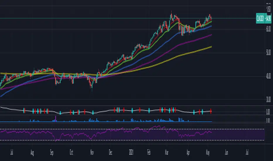
### Example Chart
*The chart below demonstrates how Fortuna Trend Predictor can help identify strong trends and avoid false breakouts by confirming signals with volume and volatility filters.*
Cerca negli script per "Exponential Moving Average"

GocchiMulti-Indicator: RSI & Moving Averages
This versatile TradingView indicator combines two essential tools for technical analysis—Relative Strength Index (RSI) and Moving Averages (MAs)—into one comprehensive solution. It is designed for traders seeking flexibility, customization, and efficiency in their charting experience.
Features:
Relative Strength Index (RSI):
Customizable RSI length.
Adjustable overbought and oversold levels.
Selectable source input (e.g., close, open, high, low).
Visual levels for overbought and oversold zones, aiding in quick trend and momentum identification.
Three Moving Averages:
Three independently customizable moving averages.
Options for Simple Moving Average (SMA) or Exponential Moving Average (EMA) for each line.
Adjustable lengths for short-, medium-, and long-term trend tracking.
Visual Enhancements:
Clear, color-coded plots for RSI and each moving average.
Overbought and oversold zones are highlighted with horizontal dotted lines.
Alerts:
Get notified when RSI crosses above the overbought level or below the oversold level.
Alerts help traders stay on top of potential market reversals or breakout opportunities.
Use Cases:
RSI Analysis: Spot overbought or oversold conditions to identify potential reversals.
Trend Following: Use moving averages to confirm trends or identify crossovers for potential entry and exit points.
Custom Strategies: Tailor the settings to fit specific trading styles, such as scalping, swing trading, or long-term investing.
This all-in-one indicator streamlines your analysis by reducing the need for multiple overlays, making your charts cleaner and more actionable. Whether you're a novice or an experienced trader, this tool provides the flexibility and insights you need to succeed in any market condition.

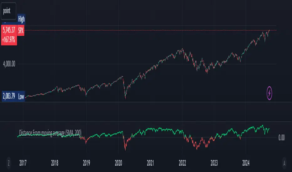
Distance From moving averageDistance From Moving Average is designed to help traders visualize the deviation of the current price from a specified moving average. Users can select from four different types of moving averages: Simple Moving Average (SMA), Exponential Moving Average (EMA), Weighted Moving Average (WMA), and Hull Moving Average (HMA).
Key Features:
User-Friendly Input Options:
Choose the type of moving average from a dropdown menu.
Set the length of the moving average, with a default value of 200.
Custom Moving Average Calculations:
The script computes the selected moving average using the appropriate mathematical formula, allowing for versatile analysis based on individual trading strategies.
Distance Calculation:
The indicator calculates the distance between the current price and the chosen moving average, providing insight into market momentum. A positive value indicates that the price is above the moving average, while a negative value shows it is below.
Visual Representation:
The distance is plotted on the chart, with color coding:
Lime: Indicates that the price is above the moving average (bullish sentiment).
Red: Indicates that the price is below the moving average (bearish sentiment).
Customization:
Users can further customize the appearance of the plotted line, enhancing clarity and visibility on the chart.
This indicator is particularly useful for traders looking to gauge market conditions and make informed decisions based on the relationship between current prices and key moving averages.
Combined EMA, SMMA, and 60-Day Cycle Indicator V2What This Script Does:
This script is designed to help traders visualize market trends and generate trading signals based on a combination of moving averages and price action. Here's a breakdown of its components and functionality:
Moving Averages:
EMAs (Exponential Moving Averages): These are indicators that smooth out price data to help identify trends. The script uses several EMAs:
200 EMA: A long-term trend indicator.
400 EMA: An even longer-term trend indicator.
55 EMA: A medium-term trend indicator.
89 EMA: Another medium-term trend indicator.
SMMA (Smoothed Moving Average): Similar to EMAs but with different smoothing. The script calculates:
21 SMMA: Short-term smoothed average.
9 SMMA: Very short-term smoothed average.
Cycle High and Low:
60-Day Cycle: The script looks back over the past 60 days to find the highest price (cycle high) and the lowest price (cycle low). These are plotted as horizontal lines on the chart.
Color-Coded Clouds:
Clouds: The script fills the area between certain EMAs with color-coded clouds to visually indicate trend conditions:
200 EMA vs. 400 EMA Cloud: Green when the 200 EMA is above the 400 EMA (bullish trend) and red when it’s below (bearish trend).
21 SMMA vs. 9 SMMA Cloud: Orange when the 21 SMMA is above the 9 SMMA and green when it’s below.
55 EMA vs. 89 EMA Cloud: Light green when the 55 EMA is above the 89 EMA and red when it’s below.
Trading Signals:
Buy Signal: This is shown when:
The price crosses above the 60-day low and
The EMAs indicate a bullish trend (e.g., the 200 EMA is above the 400 EMA and the 55 EMA is above the 89 EMA).
Sell Signal: This is shown when:
The price crosses below the 60-day high and
The EMAs indicate a bearish trend (e.g., the 200 EMA is below the 400 EMA and the 55 EMA is below the 89 EMA).
How It Helps Traders:
Trend Visualization: The colored clouds and EMA lines help you quickly see whether the market is in a bullish or bearish phase.
Trading Signals: The script provides clear visual signals (buy and sell labels) based on specific market conditions, helping you make more informed trading decisions.
In summary, this script combines several tools to help identify market trends and provide buy and sell signals based on price action relative to a 60-day high/low and the positioning of moving averages. It’s a useful tool for traders looking to visualize trends and automate some aspects of their trading strategy.
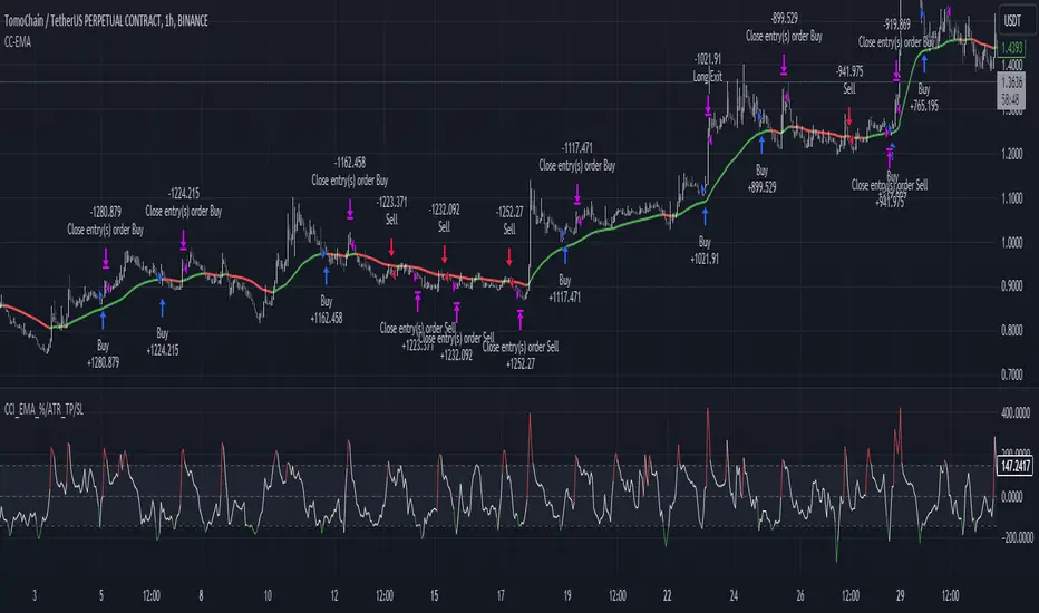
CCI+EMA Strategy with Percentage or ATR TP/SL [Alifer]This is a momentum strategy based on the Commodity Channel Index (CCI), with the aim of entering long trades in oversold conditions and short trades in overbought conditions.
Optionally, you can enable an Exponential Moving Average (EMA) to only allow trading in the direction of the larger trend. Please note that the strategy will not plot the EMA. If you want, for visual confirmation, you can add to the chart an Exponential Moving Average as a second indicator, with the same settings used in the strategy’s built-in EMA.
The strategy also allows you to set internal Stop Loss and Take Profit levels, with the option to choose between Percentage-based TP/SL or ATR-based TP/SL.
The strategy can be adapted to multiple assets and timeframes:
Pick an asset and a timeframe
Zoom back as far as possible to identify meaningful positive and negative peaks of the CCI
Set Overbought and Oversold at a rough average of the peaks you identified
Adjust TP/SL according to your risk management strategy
Like the strategy? Give it a boost!
Have any questions? Leave a comment or drop me a message.
CAUTIONARY WARNING
Please note that this is a complex trading strategy that involves several inputs and conditions. Before using it in live trading, it is highly recommended to thoroughly test it on historical data and use risk management techniques to safeguard your capital. After backtesting, it's also highly recommended to perform a first live test with a small amount. Additionally, it's essential to have a good understanding of the strategy's behavior and potential risks. Only risk what you can afford to lose .
USED INDICATORS
1 — COMMODITY CHANNEL INDEX (CCI)
The Commodity Channel Index (CCI) is a technical analysis indicator used to measure the momentum of an asset. It was developed by Donald Lambert and first published in Commodities magazine (now Futures) in 1980. Despite its name, the CCI can be used in any market and is not just for commodities. The CCI compares current price to average price over a specific time period. The indicator fluctuates above or below zero, moving into positive or negative territory. While most values, approximately 75%, fall between -100 and +100, about 25% of the values fall outside this range, indicating a lot of weakness or strength in the price movement.
The CCI was originally developed to spot long-term trend changes but has been adapted by traders for use on all markets or timeframes. Trading with multiple timeframes provides more buy or sell signals for active traders. Traders often use the CCI on the longer-term chart to establish the dominant trend and on the shorter-term chart to isolate pullbacks and generate trade signals.
CCI is calculated with the following formula:
(Typical Price - Simple Moving Average) / (0.015 x Mean Deviation)
Some trading strategies based on CCI can produce multiple false signals or losing trades when conditions turn choppy. Implementing a stop-loss strategy can help cap risk, and testing the CCI strategy for profitability on your market and timeframe is a worthy first step before initiating trades.
2 — AVERAGE TRUE RANGE (ATR)
The Average True Range (ATR) is a technical analysis indicator that measures market volatility by calculating the average range of price movements in a financial asset over a specific period of time. The ATR was developed by J. Welles Wilder Jr. and introduced in his book “New Concepts in Technical Trading Systems” in 1978.
The ATR is calculated by taking the average of the true range over a specified period. The true range is the greatest of the following:
The difference between the current high and the current low.
The difference between the previous close and the current high.
The difference between the previous close and the current low.
The ATR can be used to set stop-loss orders. One way to use ATR for stop-loss orders is to multiply the ATR by a factor (such as 2 or 3) and subtract it from the entry price for long positions or add it to the entry price for short positions. This can help traders set stop-loss orders that are more adaptive to market volatility.
3 — EXPONENTIAL MOVING AVERAGE (EMA)
The Exponential Moving Average (EMA) is a type of moving average (MA) that places a greater weight and significance on the most recent data points.
The EMA is calculated by taking the average of the true range over a specified period. The true range is the greatest of the following:
The difference between the current high and the current low.
The difference between the previous close and the current high.
The difference between the previous close and the current low.
The EMA can be used by traders to produce buy and sell signals based on crossovers and divergences from the historical average. Traders often use several different EMA lengths, such as 10-day, 50-day, and 200-day moving averages.
The formula for calculating EMA is as follows:
Compute the Simple Moving Average (SMA).
Calculate the multiplier for weighting the EMA.
Calculate the current EMA using the following formula:
EMA = Closing price x multiplier + EMA (previous day) x (1-multiplier)
STRATEGY EXPLANATION
1 — INPUTS AND PARAMETERS
The strategy uses the Commodity Channel Index (CCI) with additional options for an Exponential Moving Average (EMA), Take Profit (TP) and Stop Loss (SL).
length : The period length for the CCI calculation.
overbought : The overbought level for the CCI. When CCI crosses above this level, it may signal a potential short entry.
oversold : The oversold level for the CCI. When CCI crosses below this level, it may signal a potential long entry.
useEMA : A boolean input to enable or disable the use of Exponential Moving Average (EMA) as a filter for long and short entries.
emaLength : The period length for the EMA if it is used.
2 — CCI CALCULATION
The CCI indicator is calculated using the following formula:
(src - ma) / (0.015 * ta.dev(src, length))
src is the typical price (average of high, low, and close) and ma is the Simple Moving Average (SMA) of src over the specified length.
3 — EMA CALCULATION
If the useEMA option is enabled, an EMA is calculated with the given emaLength .
4 — TAKE PROFIT AND STOP LOSS METHODS
The strategy offers two methods for TP and SL calculations: percentage-based and ATR-based.
tpSlMethod_percentage : A boolean input to choose the percentage-based method.
tpSlMethod_atr : A boolean input to choose the ATR-based method.
5 — PERCENTAGE-BASED TP AND SL
If tpSlMethod_percentage is chosen, the strategy calculates the TP and SL levels based on a percentage of the average entry price.
tp_percentage : The percentage value for Take Profit.
sl_percentage : The percentage value for Stop Loss.
6 — ATR-BASED TP AND SL
If tpSlMethod_atr is chosen, the strategy calculates the TP and SL levels based on Average True Range (ATR).
atrLength : The period length for the ATR calculation.
atrMultiplier : A multiplier applied to the ATR to set the SL level.
riskRewardRatio : The risk-reward ratio used to calculate the TP level.
7 — ENTRY CONDITIONS
The strategy defines two conditions for entering long and short positions based on CCI and, optionally, EMA.
Long Entry: CCI crosses below the oversold level, and if useEMA is enabled, the closing price should be above the EMA.
Short Entry: CCI crosses above the overbought level, and if useEMA is enabled, the closing price should be below the EMA.
8 — TP AND SL LEVELS
The strategy calculates the TP and SL levels based on the chosen method and updates them dynamically.
For the percentage-based method, the TP and SL levels are calculated as a percentage of the average entry price.
For the ATR-based method, the TP and SL levels are calculated using the ATR value and the specified multipliers.
9 — EXIT CONDITIONS
The strategy defines exit conditions for both long and short positions.
If there is a long position, it will be closed either at TP or SL levels based on the chosen method.
If there is a short position, it will be closed either at TP or SL levels based on the chosen method.
Additionally, positions will be closed if CCI crosses back above oversold in long positions or below overbought in short positions.
10 — PLOTTING
The script plots the CCI line along with overbought and oversold levels as horizontal lines.
The CCI line is colored red when above the overbought level, green when below the oversold level, and white otherwise.
The shaded region between the overbought and oversold levels is plotted as well.
Moving Average Multitool CrossoverAs per request, this is a moving average crossover version of my original moving average multitool script .
It allows you to easily access and switch between different types of moving averages, without having to continuously add and remove different moving averages from your chart. This should make backtesting moving average crossovers much, much more easier. It also has the option to show buy and sell signals for the crossovers of the chosen moving averages.
It contains the following moving averages:
Exponential Moving Average (EMA)
Simple Moving Average (SMA)
Weighted Moving Average (WMA)
Double Exponential Moving Average (DEMA)
Triple Exponential Moving Average (TEMA)
Triangular Moving Average (TMA)
Volume-Weighted Moving Average (VWMA)
Smoothed Moving Average (SMMA)
Hull Moving Average (HMA)
Least Squares Moving Average (LSMA)
Kijun-Sen line from the Ichimoku Kinko-Hyo system (Kijun)
McGinley Dynamic (MD)
Rolling Moving Average (RMA)
Jurik Moving Average (JMA)
Arnaud Legoux Moving Average (ALMA)
Vector Autoregression Moving Average (VAR)
Welles Wilder Moving Average (WWMA)
Sine Weighted Moving Average (SWMA)
Leo Moving Average (LMA)
Variable Index Dynamic Average (VIDYA)
Fractal Adaptive Moving Average (FRAMA)
Variable Moving Average (VAR)
Geometric Mean Moving Average (GMMA)
Corrective Moving Average (CMA)
Moving Median (MM)
Quick Moving Average (QMA)
Kaufman's Adaptive Moving Average (KAMA)
Volatility-Adjusted Moving Average (VAMA)
Modular Filter (MF)

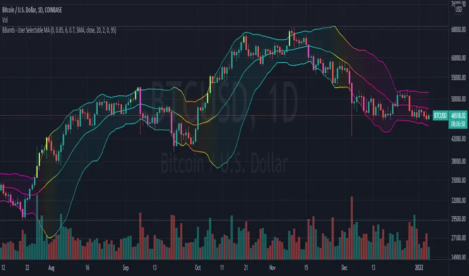
Bollinger Bands With User Selectable MABollinger Bands with user selection options to calculate the moving average basis and bands from a variety of different moving averages.
The user selects their choice of moving average, and the bands automatically adjust. The user may select a MA that reacts faster to volatility or slower/smoother.
Added additional options to color the bands or basis based on the current trend and alternate candle colors for band touches. Options:
REACT SLOW/SMOOTH TO VOLATILITY
simple moving average (Regular Bollinger Bands)
REACT SMOOTH TO VOLATILITY
exponential moving average (EMA Bollinger Bands)
weighted moving average (Weighted MA Bollinger Bands)
exponential hull moving average (Hull Bollinger Bands with better smoothing)
HIGHLY ADJUSTABLE TO VOLATILITY
Arnaud Legoux Moving average (ALMA Bollinger Bands)
Note: 0.85 ALMA default for more smoothing, set offset=1 to turn off smoothing
REACT HARSH TO VOLATILITY
least squares moving average (Least Squares Bollinger Bands)
REACT VERY FAST TO VOLATILITY
hull moving average (Hull Bollinger Bands or Hullinger Bands)
VALUE ADDED: This script is unique in that no other Bollinger Bands indicator offers a user selection for moving average, and some of the options do not exist yet as Bollinger Bands indicators.
Definitions:
Bollinger Bands: A Bollinger Band® is a technical analysis tool defined by a set of trendlines plotted two standard deviations (positively and negatively) away from a simple moving average (SMA) of a security's price, but which can be adjusted to user preferences.
Exponential Bollinger Bands: The most important characteristics of the Exponential Bollinger Bands indicator are: When the market is flat, the bands will stay much closer to prices. When the volatility is high, the bands move away from prices faster.
Hull Bollinger Bands: Bollinger Bands calculated by Hull moving average, rather than simple moving average or ema. The Hull Moving Average (HMA), developed by Alan Hull, is an extremely fast and smooth moving average. In fact, the HMA almost eliminates lag altogether and manages to improve smoothing at the same time.
Exponential Hull Bollinger Bands: Bollinger Bands calculated by Exponential Hull moving average, rather than simple moving average or ema. The Exponential Hull Moving Average is similar to the standard Hull MA, but with superior smoothing. The standard Hull Moving Average is derived from the weighted moving average (WMA). As other moving average built from weighted moving averages it has a tendency to exaggerate price movement.
Weighted Moving Average Bollinger Bands: A Weighted Moving Average (WMA) is similar to the simple moving average (SMA), except the WMA adds significance to more recent data points.
Arnaud Legoux Moving Average Bollinger Bands: ALMA removes small price fluctuations and enhances the trend by applying a moving average twice, once from left to right, and once from right to left. At the end of this process the phase shift (price lag) commonly associated with moving averages is significantly reduced. Zero-phase digital filtering reduces noise in the signal. Conventional filtering reduces noise in the signal, but adds a delay.
Least Squares Bollinger Bands: The indicator is based on sum of least squares method to find a straight line that best fits data for the selected period. The end point of the line is plotted and the process is repeated on each succeeding period.
Multiple EMAAn exponential moving average (EMA) is a type of moving average (MA) that places a greater weight and significance on the most recent data points. The exponential moving average is also referred to as the exponentially weighted moving average. An exponentially weighted moving average reacts more significantly to recent price changes than a simple moving average (SMA), which applies an equal weight to all observations in the period.
The EMA is a moving average that places a greater weight and significance on the most recent data points.
Like all moving averages, this technical indicator is used to produce buy and sell signals based on crossovers and divergences from the historical average.
Traders often use several different EMA lengths, such as 10-day, 50-day, and 200-day moving averages.
Points to remember:
Exponential moving averages are more sensitive to the recent price
EMA can signal good trades, but it can also keep you out of bad trades
EMA offers dynamic support and resistance levels, which is good for trailing Stop Loss
The EMA slope shape has hidden secrets
The rules for the EMA trading strategy can be modified to fit your own trading needs. We don’t claim this to be hard rules, but they are good on their own to make for a great trading strategy. Make sure you first test out the EMA strategy on a paper trading account before you risk any of your hard-earned money
Displaced MAsDisplaced Moving Averages with Customizable Bands
Overview
The "Displaced Moving Averages with Customizable Bands" indicator is a powerful and versatile tool designed to provide a comprehensive view of price action in relation to various moving averages (MAs) and their volatility. It offers a high degree of customization, allowing traders to tailor the indicator to their specific needs and trading styles. The indicator features a primary moving average with multiple configurable percentage-based displacement bands. It also includes additional moving averages with standard deviation bands for a more in-depth analysis of different timeframes.
Key Features
Multiple Moving Average Types:
Choose from a wide range of popular moving average types for the primary MA calculation:
WMA (Weighted Moving Average)
EMA (Exponential Moving Average)
SMA (Simple Moving Average)
HMA (Hull Moving Average)
VWAP (Volume-Weighted Average Price)
Smoothed VWAP
Rolling VWAP
The flexibility to select the most appropriate MA type allows you to adapt the indicator to different market conditions and trading strategies.
Smoothed VWAP with Customizable Smoothing:
When "Smoothed VWAP" is selected, you can further refine it by choosing a smoothing type: SMA, EMA, WMA, or HMA.
Customize the smoothing period based on the chart's timeframe (1H, 4H, D, W) or use a default period. This feature offers fine-grained control over the responsiveness of the VWAP calculation.
Rolling VWAP with Adjustable Lookback:
The "Rolling VWAP" option calculates the VWAP over a user-defined lookback period.
Customize the lookback length for different timeframes (1H, 4H, D, W) or use a default period. This provides a dynamic VWAP calculation that adapts to the chosen timeframe.
Customizable Lookback Lengths:
Define the lookback period for the primary moving average calculation.
Tailor the lookback lengths for different timeframes (1H, 4H, D, W) or use a default value.
This allows you to adjust the sensitivity of the MA to recent price action based on the timeframe you are analyzing. Also has inputs for 5m, and 15m timeframes.
Percentage-Based Displacement Bands:
The core feature of this indicator is the ability to plot multiple displacement bands above and below the primary moving average.
These bands are calculated as a percentage offset from the MA, providing a clear visualization of price deviations.
Visibility Toggles: Independently show or hide each band (+/- 2%, 5%, 7%, 10%, 15%, 20%, 25%, 30%, 40%, 50%, 60%, 70%).
Customizable Colors: Assign unique colors to each band for easy visual identification.
Adjustable Multipliers: Fine-tune the percentage displacement for each band using individual multiplier inputs.
The bands are useful for identifying potential support and resistance levels, overbought/oversold conditions, and volatility expansions/contractions.
Labels for Displacement Bands:
The indicator displays labels next to each plotted band, clearly indicating the percentage displacement (e.g., "+7%", "-15%").
Customize the label text color for optimal visibility.
The labels can be horizontally offset by a user-defined number of bars.
Additional Moving Averages with Standard Deviation Bands:
The indicator includes three additional moving averages, each with upper and lower standard deviation bands. These are designed to provide insights into volatility on different timeframes.
Timeframe Selection: Choose the timeframes for these additional MAs (e.g., Weekly, 4-Hour, Daily).
Sigma (Standard Deviation Multiplier): Adjust the standard deviation multiplier for each MA.
MA Length: Set the lookback period for each additional MA.
Visibility Toggles: Show or hide the lower band of MA1, the middle/upper/lower bands of MA2, and the bands of MA3.
4h Bollinger Middle MA is unticked by default to provide a less cluttered chart
These additional MAs are particularly useful for multi-timeframe analysis and identifying potential trend reversals or volatility shifts.
How to Use
Add the indicator to your TradingView chart.
Customize the settings:
Select the desired Moving Average Type for the primary MA.
If using Smoothed VWAP, choose the Smoothing Type and adjust the Smoothing Period for different timeframes.
If using Rolling VWAP, adjust the Lookback Length for different timeframes.
Set the Lookback Length for the primary MA for different timeframes.
Toggle the visibility of the Displacement Bands and adjust their Colors and Multipliers.
Customize the Label Text Color and Offset.
Configure the Timeframes, Sigma, and MA Length for the additional moving averages.
Toggle the visibility of the additional MA bands.
Interpret the plotted lines and bands:
Primary MA: Represents the average price over the selected lookback period, calculated using the chosen MA type.
Displacement Bands: Indicate potential support and resistance levels, overbought/oversold conditions, and volatility ranges. Price trading outside these bands may signal significant deviations from the average.
Additional MAs with Standard Deviation Bands: Provide insights into volatility on different timeframes. Wider bands suggest higher volatility, while narrower bands indicate lower volatility.
Potential Trading Applications
Trend Identification: Use the primary MA to identify the overall trend direction.
Support and Resistance: The displacement bands can act as dynamic support and resistance levels.
Overbought/Oversold: Price reaching the outer displacement bands may suggest overbought or oversold conditions, potentially indicating a pullback or reversal.
Volatility Analysis: The standard deviation bands of the additional MAs can help assess volatility on different timeframes.
Multi-Timeframe Analysis: Combine the primary MA with the additional MAs to gain a broader perspective on price action across multiple timeframes.
Entry and Exit Signals: Use the interaction of price with the MA and bands to generate potential entry and exit signals. For example, a bounce off a lower band could be a buy signal, while a rejection from an upper band could be a sell signal.
Disclaimer
This indicator is for informational and educational purposes only and should not be considered financial advice. Trading involves risk, and past performance is not indicative of future results. Always conduct thorough research and consider your risk tolerance before making any trading decisions.
Enjoy using the "Displaced Moving Averages with Customizable Bands" indicator!

Fear/Greed Zone Reversals [UAlgo]The "Fear/Greed Zone Reversals " indicator is a custom technical analysis tool designed for TradingView, aimed at identifying potential reversal points in the market based on sentiment zones characterized by fear and greed. This indicator utilizes a combination of moving averages, standard deviations, and price action to detect when the market transitions from extreme fear to greed or vice versa. By identifying these critical turning points, traders can gain insights into potential buy or sell opportunities.
🔶 Key Features
Customizable Moving Averages: The indicator allows users to select from various types of moving averages (SMA, EMA, WMA, VWMA, HMA) for both fear and greed zone calculations, enabling flexible adaptation to different trading strategies.
Fear Zone Settings:
Fear Source: Select the price data point (e.g., close, high, low) used for Fear Zone calculations.
Fear Period: This defines the lookback window for calculating the Fear Zone deviation.
Fear Stdev Period: This sets the period used to calculate the standard deviation of the Fear Zone deviation.
Greed Zone Settings:
Greed Source: Select the price data point (e.g., close, high, low) used for Greed Zone calculations.
Greed Period: This defines the lookback window for calculating the Greed Zone deviation.
Greed Stdev Period: This sets the period used to calculate the standard deviation of the Greed Zone deviation.
Alert Conditions: Integrated alert conditions notify traders in real-time when a reversal in the fear or greed zone is detected, allowing for timely decision-making.
🔶 Interpreting Indicator
Greed Zone: A Greed Zone is highlighted when the price deviates significantly above the chosen moving average. This suggests market sentiment might be leaning towards greed, potentially indicating a selling opportunity.
Fear Zone Reversal: A Fear Zone is highlighted when the price deviates significantly below the chosen moving average of the selected price source. This suggests market sentiment might be leaning towards fear, potentially indicating a buying opportunity. When the indicator identifies a reversal from a fear zone, it suggests that the market is transitioning from a period of intense selling pressure to a more neutral or potentially bullish state. This is typically indicated by an upward arrow (▲) on the chart, signaling a potential buy opportunity. The fear zone is characterized by high price volatility and overselling, making it a crucial point for traders to consider entering the market.
Greed Zone Reversal: Conversely, a Greed Zone is highlighted when the price deviates significantly above the chosen moving average. This suggests market sentiment might be leaning towards greed, potentially indicating a selling opportunity. When the indicator detects a reversal from a greed zone, it indicates that the market may be moving from an overbought condition back to a more neutral or bearish state. This is marked by a downward arrow (▼) on the chart, suggesting a potential sell opportunity. The greed zone is often associated with overconfidence and high buying activity, which can precede a market correction.
🔶 Why offer multiple moving average types?
By providing various moving average types (SMA, EMA, WMA, VWMA, HMA) , the indicator offers greater flexibility for traders to tailor the indicator to their specific trading strategies and market preferences. Different moving averages react differently to price data and can produce varying signals.
SMA (Simple Moving Average): Provides an equal weighting to all data points within the specified period.
EMA (Exponential Moving Average): Gives more weight to recent data points, making it more responsive to price changes.
WMA (Weighted Moving Average): Allows for custom weighting of data points, providing more flexibility in the calculation.
VWMA (Volume Weighted Moving Average): Considers both price and volume data, giving more weight to periods with higher trading volume.
HMA (Hull Moving Average): A combination of weighted moving averages designed to reduce lag and provide a smoother curve.
Offering multiple options allows traders to:
Experiment: Traders can try different moving averages to see which one produces the most accurate signals for their specific market.
Adapt to different market conditions: Different market conditions may require different moving average types. For example, a fast-moving market might benefit from a faster moving average like an EMA, while a slower-moving market might be better suited to a slower moving average like an SMA.
Personalize: Traders can choose the moving average that best aligns with their personal trading style and risk tolerance.
In essence, providing a variety of moving average types empowers traders to create a more personalized and effective trading experience.
🔶 Disclaimer
Use with Caution: This indicator is provided for educational and informational purposes only and should not be considered as financial advice. Users should exercise caution and perform their own analysis before making trading decisions based on the indicator's signals.
Not Financial Advice: The information provided by this indicator does not constitute financial advice, and the creator (UAlgo) shall not be held responsible for any trading losses incurred as a result of using this indicator.
Backtesting Recommended: Traders are encouraged to backtest the indicator thoroughly on historical data before using it in live trading to assess its performance and suitability for their trading strategies.
Risk Management: Trading involves inherent risks, and users should implement proper risk management strategies, including but not limited to stop-loss orders and position sizing, to mitigate potential losses.
No Guarantees: The accuracy and reliability of the indicator's signals cannot be guaranteed, as they are based on historical price data and past performance may not be indicative of future results.

Adaptive MA-Bollinger HistogramVisualize two of your favorite moving averages in a fun new way.
This script calculates the distance (or difference) between the price and two moving averages of your choosing and then creates two histograms.
The two histograms are plotted inversely, so if the price is over both moving averages, one will be positive above the centerline while the other still positive will be below the centerline.
(In a future update you will have the option to have them both positive at the same time)
Next, what it does is apply Bollinger Bands (optional) to each of the histograms.
This creates a very interesting effect that can highlight areas of interest you may miss with other indicators.
You have plenty of options for coloring, the type of moving average, Bollinger Band length, and toggling features on and off.
Give it a few minutes of your time to study, and see what information you can learn from watching this indicator by comparing it with the chart.
Here is a full user guide:
Adaptive MA-Bollinger Histogram Indicator User Guide
Welcome to the user guide for the **Adaptive MA-Bollinger Histogram** indicator. This custom indicator is designed to help traders analyze trends and potential reversals in a financial instrument's price movements. The indicator combines two Moving Averages (MA) and Bollinger Bands to provide valuable insights into market conditions.
### Indicator Overview
The Adaptive MA-Bollinger Histogram indicator comprises the following components:
1. **Moving Averages (MA1 and MA2):** The indicator uses two moving averages, namely MA1 and MA2, to track different time periods. MA1 has a user-defined length (default: 50) and MA2 has a longer user-defined length (default: 100). These moving averages can be calculated using different methods such as Simple Moving Average (SMA), Exponential Moving Average (EMA), Weighted Moving Average (WMA), Volume Weighted Moving Average (VWMA), or Smoothed Moving Average (RMA).
2. **Histograms:** The indicator displays histograms based on the differences between the price source and the respective moving averages. Positive values of the histogram for MA1 are plotted in one color (default: green), while negative values are plotted in another color (default: red). Similarly, positive values of the histogram for MA2 are plotted in one color (default: blue), while negative values are plotted in another color (default: yellow). It's important to note that the histogram for MA1 is plotted positively, while the histogram for MA2 is plotted inversely.
3. **Bollinger Bands:** The indicator also features Bollinger Bands calculated based on the differences between the price source and the respective moving averages (dist1 and dist2). Bollinger Bands consist of three lines: the middle band, upper band, and lower band. These bands help visualize the potential volatility and overbought/oversold levels of the instrument's price.
### Understanding the Indicator
- **Histograms:** The histograms highlight the divergence between the price and the two moving averages. When the histogram for MA1 is positive, it indicates that the price is above the MA1. Conversely, when the histogram for MA1 is negative, it suggests that the price is below the MA1. Similarly, the histogram for MA2 is plotted inversely.
- **Bollinger Bands:** The Bollinger Bands consist of three lines. The middle band represents the moving average (MA1 or MA2), while the upper and lower bands are calculated based on the standard deviation of the differences between the price source and the moving average. The bands expand during periods of higher volatility and contract during periods of lower volatility.
### Possible Trading Ideas
1. **Trend Confirmation:** When the histograms for both MA1 and MA2 are consistently positive, it may indicate a strong bullish trend. Conversely, when both histograms are consistently negative, it may suggest a strong bearish trend.
2. **Divergence:** Divergence between price and the histograms could signal potential reversals. For example, if the price is making new highs while the histogram is declining, it might indicate a bearish divergence and a possible upcoming trend reversal.
3. **Bollinger Bands Squeeze:** A narrowing of the Bollinger Bands indicates lower volatility and often precedes a significant price movement. Traders might consider a potential breakout trade when the bands start to expand again.
4. **Overbought/Oversold Levels:** Prices touching or exceeding the upper Bollinger Band could suggest overbought conditions, while prices touching or falling below the lower Bollinger Band could indicate oversold conditions. Traders might look for reversals or corrections in such scenarios.
### Customization
- You can adjust the parameters such as MA lengths, Bollinger Bands length, width, and colors to suit your preferences and trading strategy.
### Conclusion
The **Adaptive MA-Bollinger Histogram** indicator provides a comprehensive view of price trends, divergences, and potential reversal points. Traders can use the information from this indicator to make informed decisions in their trading strategies. However, like any technical tool, it's recommended to combine this indicator with other forms of analysis and risk management techniques for optimal results.

MA DerivativesMA Derivatives basicly using Ichimoku Cloud and some additional moving averages for traders.
A. ICHIMOKU
Tenkan-sen (Conversion Line): (9-period high + 9-period low)/2
On a daily chart , this line is the midpoint of the 9-day high-low range, which is almost two weeks.
Kijun-sen (Base Line): (26-period high + 26-period low)/2
On a daily chart , this line is the midpoint of the 26-day high-low range, which is almost one month.
Senkou Span A (Leading Span A): (Conversion Line + Base Line)/2
This is the midpoint between the Conversion Line and the Base Line. The Leading Span A forms one of the two Cloud boundaries. It is referred to as “Leading” because it is plotted 26 periods in the future and forms the faster Cloud boundary.
Senkou Span B (Leading Span B): (52-period high + 52-period low)/2
On the daily chart , this line is the midpoint of the 52-day high-low range, which is a little less than 3 months. The default calculation setting is 52 periods, but it can be adjusted. This value is plotted 26 periods in the future and forms the slower Cloud boundary.
Chikou Span: Represents the closing price and is plotted 26 days back.
Kumo Cloud: Kumo cloud between Senkuo Span A and Senkou Span B lines. It can be green or red. Color can be change with the trend.
You can use Ichimoku for buy&sell strategy
For Buying Strategy
- Tenkansen (Conversion Line) should crossover Kijunsen (Base line) above the highest line of cloud
- Price should be above the highest line of cloud
- Chikouspan should be above the cloud
For Selling Strategy
- Kijunsen (Base Line) should crossover Tenkansen (Conversion Line) below the lowest line of cloud
- Price should be below the lowest line of cloud
- Chikouspan should be below the cloud
B. SIMPLE MOVING AVERAGES
The indicator has some of Simple Moving Averages
It includes:
-Simple Moving Average 50
-Simple Moving Average 100
-Simple Moving Average 200
C. EXPONENTIAL MOVING AVERAGES
The indicator has some of Simple Moving Averages
It includes:
-Exponential Moving Average 9
-Exponential Moving Average 21
-Exponential Moving Average 50
D. BOLLINGER BAND
Bollinger Bands are a type of price envelope developed by John BollingerOpens in a new window. (Price envelopes define upper and lower price range levels.) Bollinger Bands are envelopes plotted at a standard deviation level above and below a simple moving average of the price. Because the distance of the bands is based on standard deviation, they adjust to volatility swings in the underlying price.
Bollinger Bands use 2 parameters, Period and Standard Deviations, StdDev. The default values are 20 for period, and 2 for standard deviations, although you may customize the combinations.
Bollinger bands help determine whether prices are high or low on a relative basis. They are used in pairs, both upper and lower bands and in conjunction with a moving average. Further, the pair of bands is not intended to be used on its own. Use the pair to confirm signals given with other indicators.
How this indicator works
When the bands tighten during a period of low volatility, it raises the likelihood of a sharp price move in either direction. This may begin a trending move. Watch out for a false move in opposite direction which reverses before the proper trend begins.
When the bands separate by an unusual large amount, volatility increases and any existing trend may be ending.
Prices have a tendency to bounce within the bands' envelope, touching one band then moving to the other band. You can use these swings to help identify potential profit targets. For example, if a price bounces off the lower band and then crosses above the moving average, the upper band then becomes the profit target.
Price can exceed or hug a band envelope for prolonged periods during strong trends. On divergence with a momentum oscillator, you may want to do additional research to determine if taking additional profits is appropriate for you.
A strong trend continuation can be expected when the price moves out of the bands. However, if prices move immediately back inside the band, then the suggested strength is negated.
Calculation
First, calculate a simple moving average. Next, calculate the standard deviation over the same number of periods as the simple moving average. For the upper band, add the standard deviation to the moving average. For the lower band, subtract the standard deviation from the moving average.
Typical values used:
Short term: 10 day moving average, bands at 1.5 standard deviations. (1.5 times the standard dev. +/- the SMA)
Medium term: 20 day moving average, bands at 2 standard deviations.
Long term: 50 day moving average, bands at 2.5 standard deviations.
E. ADJUSTABLE MOVING AVERAGES
And this script has also 2 adjustable moving average
- 1 Adjustable Simple Moving Average
- 1 Adjustable Exponential Moving Average
You can just change the length for using this tool.

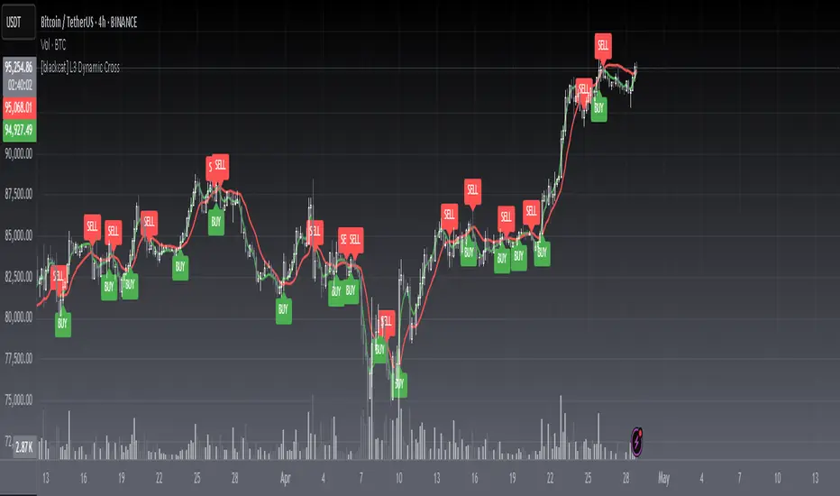
[blackcat] L3 Dynamic CrossOVERVIEW
The L3 Dynamic Cross indicator is a powerful tool designed to assist traders in identifying potential buy and sell opportunities through the use of dynamic moving averages. This versatile script offers a wide range of customizable options, allowing users to tailor the moving averages to their specific needs and preferences. By providing clear visual cues and generating precise crossover signals, it helps traders make informed decisions about market trends and potential entry/exit points 📈💹.
FEATURES
Multiple Moving Average Types:
Simple Moving Average (SMA): Provides a straightforward average of prices over a specified period.
Exponential Moving Average (EMA): Gives more weight to recent prices, making it responsive to new information.
Weighted Moving Average (WMA): Assigns weights to all prices within the look-back period, giving more importance to recent prices.
Volume Weighted Moving Average (VWMA): Incorporates volume data to provide a more accurate representation of price movements.
Smoothed Moving Average (SMMA): Averages out fluctuations to create a smoother trend line.
Double Exponential Moving Average (DEMA): Reduces lag by applying two layers of exponential smoothing.
Triple Exponential Moving Average (TEMA): Further reduces lag with three layers of exponential smoothing.
Hull Moving Average (HullMA): Combines weighted moving averages to minimize lag and noise.
Super Smoother Moving Average (SSMA): Uses a sophisticated algorithm to smooth out price data while preserving trend direction.
Zero-Lag Exponential Moving Average (ZEMA): Eliminates lag entirely by adjusting the calculation method.
Triangular Moving Average (TMA): Applies a double smoothing process to reduce volatility and enhance trend identification.
Customizable Parameters:
Length: Adjust the period for both fast and slow moving averages to match your trading style.
Source: Select different price sources such as close, open, high, or low for more nuanced analysis.
Visual Representation:
Fast MA: Displayed as a green line representing shorter-term trends.
Slow MA: Shown as a red line indicating longer-term trends.
Crossover Signals:
Generate buy ('BUY') and sell ('SELL') labels based on crossover events between the fast and slow moving averages 🏷️.
Clear visual cues help traders quickly identify potential entry and exit points.
Alert Functionality:
Receive real-time notifications when crossover conditions are met, ensuring timely action 🔔.
Customizable alert messages for personalized trading strategies.
Advanced Trade Management:
Support for pyramiding levels allows traders to manage multiple positions effectively.
Fine-tune your risk management by setting the number of allowed trades per signal.
HOW TO USE
Adding the Indicator:
Open your TradingView chart and go to the indicators list.
Search for L3 Dynamic Cross and add it to your chart.
Configuring Settings:
Choose your desired Moving Average Type from the dropdown menu.
Adjust the Fast MA Length and Slow MA Length according to your trading timeframe.
Select appropriate Price Sources for both fast and slow moving averages.
Monitoring Signals:
Observe the plotted lines on the chart to track short-term and long-term trends.
Look for buy and sell labels that indicate potential trade opportunities.
Setting Up Alerts:
Enable alerts based on crossover conditions to receive instant notifications.
Customize alert messages to suit your trading plan.
Managing Positions:
Utilize the pyramiding feature to handle multiple entries and exits efficiently.
Keep track of your position sizes relative to the defined pyramiding levels.
Combining with Other Tools:
Integrate this indicator with other technical analysis tools for confirmation.
Use additional filters like volume, RSI, or MACD to enhance decision-making accuracy.
LIMITATIONS
Market Conditions: The effectiveness of the indicator may vary in highly volatile or sideways markets. Be cautious during periods of low liquidity or sudden price spikes 🌪️.
Parameter Sensitivity: Different moving average types and lengths can produce varying results. Experiment with settings to find what works best for your asset class and timeframe.
False Signals: Like any technical indicator, false signals can occur. Always confirm signals with other forms of analysis before executing trades.
NOTES
Historical Data: Ensure you have enough historical data loaded into your chart for accurate moving average calculations.
Backtesting: Thoroughly backtest the indicator on various assets and timeframes using demo accounts before deploying it in live trading environments 🔍.
Customization: Feel free to adjust colors, line widths, and label styles to better fit your chart aesthetics and personal preferences.
EXAMPLE STRATEGIES
Trend Following: Use the indicator to ride trends by entering positions when the fast MA crosses above/below the slow MA and exiting when the opposite occurs.
Mean Reversion: Identify overbought/oversold conditions by combining the indicator with oscillators like RSI or Stochastic. Enter counter-trend positions when the moving averages diverge significantly from the mean.
Scalping: Apply tight moving average settings to capture small, quick profits in intraday trading. Combine with volume indicators to filter out weak signals.
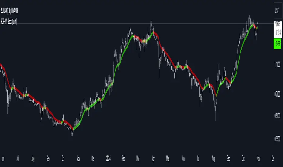
PDF Smoothed Moving Average [BackQuant]PDF Smoothed Moving Average
Introducing BackQuant’s PDF Smoothed Moving Average (PDF-MA) — an innovative trading indicator that applies Probability Density Function (PDF) weighting to moving averages, creating a unique, trend-following tool that offers adaptive smoothing to price movements. This advanced indicator gives traders an edge by blending PDF-weighted values with conventional moving averages, helping to capture trend shifts with enhanced clarity.
Core Concept: Probability Density Function (PDF) Smoothing
The Probability Density Function (PDF) provides a mathematical approach to applying adaptive weighting to data points based on a specified variance and mean. In the PDF-MA indicator, the PDF function is used to weight price data, adding a layer of probabilistic smoothing that enhances the detection of trend strength while reducing noise.
The PDF weights are controlled by two key parameters:
Variance: Determines the spread of the weights, where higher values spread out the weighting effect, providing broader smoothing.
Mean : Centers the weights around a particular price value, influencing the trend’s directionality and sensitivity.
These PDF weights are applied to each price point over the chosen period, creating an adaptive and smooth moving average that more closely reflects the underlying price trend.
Blending PDF with Standard Moving Averages
To further improve the PDF-MA, this indicator combines the PDF-weighted average with a traditional moving average, selected by the user as either an Exponential Moving Average (EMA) or Simple Moving Average (SMA). This blended approach leverages the strengths of each method: the responsiveness of PDF smoothing and the robustness of conventional moving averages.
Smoothing Method: Traders can choose between EMA and SMA for the additional moving average layer. The EMA is more responsive to recent prices, while the SMA provides a consistent average across the selected period.
Smoothing Period: Controls the length of the lookback period, affecting how sensitive the average is to price changes.
The result is a PDF-MA that provides a reliable trend line, reflecting both the PDF weighting and traditional moving average values, ideal for use in trend-following and momentum-based strategies.
Trend Detection and Candle Coloring
The PDF-MA includes a built-in trend detection feature that dynamically colors candles based on the direction of the smoothed moving average:
Uptrend: When the PDF-MA value is increasing, the trend is considered bullish, and candles are colored green, indicating potential buying conditions.
Downtrend: When the PDF-MA value is decreasing, the trend is considered bearish, and candles are colored red, signaling potential selling or shorting conditions.
These color-coded candles provide a quick visual reference for the trend direction, helping traders make real-time decisions based on the current market trend.
Customization and Visualization Options
This indicator offers a range of customization options, allowing traders to tailor it to their specific preferences and trading environment:
Price Source : Choose the price data for calculation, with options like close, open, high, low, or HLC3.
Variance and Mean : Fine-tune the PDF weighting parameters to control the indicator’s sensitivity and responsiveness to price data.
Smoothing Method : Select either EMA or SMA to customize the conventional moving average layer used in conjunction with the PDF.
Smoothing Period : Set the lookback period for the moving average, with a longer period providing more stability and a shorter period offering greater sensitivity.
Candle Coloring : Enable or disable candle coloring based on trend direction, providing additional clarity in identifying bullish and bearish phases.
Trading Applications
The PDF Smoothed Moving Average can be applied across various trading strategies and timeframes:
Trend Following : By smoothing price data with PDF weighting, this indicator helps traders identify long-term trends while filtering out short-term noise.
Reversal Trading : The PDF-MA’s trend coloring feature can help pinpoint potential reversal points by showing shifts in the trend direction, allowing traders to enter or exit positions at optimal moments.
Swing Trading : The PDF-MA provides a clear trend line that swing traders can use to capture intermediate price moves, following the trend direction until it shifts.
Final Thoughts
The PDF Smoothed Moving Average is a highly adaptable indicator that combines probabilistic smoothing with traditional moving averages, providing a nuanced view of market trends. By integrating PDF-based weighting with the flexibility of EMA or SMA smoothing, this indicator offers traders an advanced tool for trend analysis that adapts to changing market conditions with reduced lag and increased accuracy.
Whether you’re trading trends, reversals, or swings, the PDF-MA offers valuable insights into the direction and strength of price movements, making it a versatile addition to any trading strategy.
Deviation Adjusted MA Overview
The Deviation Adjusted MA is a custom indicator that enhances traditional moving average techniques by introducing a volatility-based adjustment. This adjustment is implemented by incorporating the standard deviation of price data, making the moving average more adaptive to market conditions. The key feature is the combination of a customizable moving average (MA) type and the application of deviation percentage to modify its responsiveness. Additionally, a smoothing layer is applied to reduce noise, improving signal clarity.
Key Components
Customizable Moving Averages
The script allows the user to select from four different types of moving averages:
Simple Moving Average (SMA): A basic average of the closing prices over a specified period.
Exponential Moving Average (EMA): Gives more weight to recent prices, making it more responsive to recent price changes.
Weighted Moving Average (WMA): Weights prices differently, favoring more recent ones but in a linear progression.
Volume-Weighted Moving Average (VWMA): Adjusts the average by trading volume, placing more weight on high-volume periods.
Standard Deviation Calculation
The script calculates the standard deviation of the closing prices over the selected maLength period.
Standard deviation measures the dispersion or volatility of price movements, giving a sense of market volatility.
Deviation Percentage and Adjustment
Deviation Percentage is calculated by dividing the standard deviation by the base moving average and multiplying by 100 to express it as a percentage.
The base moving average is adjusted by this deviation percentage, making the indicator responsive to changes in volatility. The result is a more dynamic moving average that adapts to market conditions.
The parameter devMultiplier is available to scale this adjustment, allowing further fine-tuning of sensitivity.
Smoothing the Adjusted Moving Average
After adjusting the moving average based on deviation, the script applies an additional Exponential Moving Average (EMA) with a length defined by the smoothingLength input.
This EMA serves as a smoothing filter to reduce the noise that could arise from the raw adjustments of the moving average. The smoothing makes trend recognition more consistent and removes short-term fluctuations that could otherwise distort the signal.
Use cases
The Deviation Adjusted MA indicator serves as a dynamic alternative to traditional moving averages by adjusting its sensitivity based on volatility. The script offers extensive customization options through the selection of moving average type and the parameters controlling smoothing and deviation adjustments.
By applying these adjustments and smoothing, the script enables users to better track trends and price movements, while providing a visual cue for changes in market sentiment.

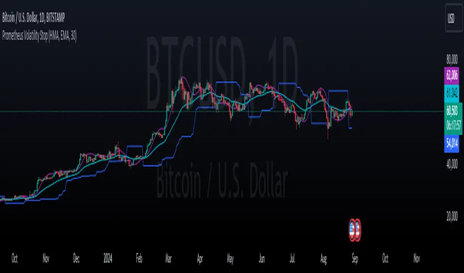
Prometheus Volatility StopThe Prometheus Volatility Stop is an indicator designed to give you a moving risk metric along with a custom Moving Average cross. After a calculation of the annualized volatility for the specified lookback period we determine bullish or bearish from the moving averages and plot the Volatility Stop accordingly.
User Input:
A user can select from Hull Moving Average, Exponential Moving average, Simple Moving Average, the Moving Average used in RSI, and Weighted Moving Average. The default is Hull Moving Average and Exponential Moving average.
A user can also specify the lookback period. The default is 30.
A user may also turn off the plots for the Moving Averages.
The reason for this approach is to be more original from the traditional Volatility Stop.
Calculation:
The Historical Volatility is calculated by taking the standard deviation of the log returns for the specified period and then annualizing it.
hv = ta.stdev(math.log(close / close ), lkb) * math.sqrt(252/5)
Then the Volatility Stop is calculated as follows:
recent_max = ta.highest(close, lkb)
recent_min = ta.lowest(close, lkb)
hv_stop = ma_2 > ma_1 ? recent_max + hv : recent_min - hv
When the second selected moving average is greater than the first, which signals bearishness, the historical volatility gets added to the high of that period. When the moving averages signal bullish the historical volatility gets subtracted from the low of that period.
Here is an example on NASDAQ:ARM :
After the first crossover, bullish signal, price runs for some time. As we get higher and higher so does the Volatility Stop. At the highs before a bearish crossover the price hits and closes at the Volatility Stop. Providing what could be an exit from a strong run up.
Intra-day example on NASDAQ:QQQ :
We see that in the early bearish move price goes on to hit the Volatility Stop before the trend switches.
We also see that in the failed long. The price action throughout the rest of the day, while not providing in profit stop outs, do provide fine directional alerts.
All those examples have been done with the default settings. Upon changing Moving Average One to a WMA and Moving Average Two to an SMA, as well as the lookback to 75. We see this quickly can become a simple trend follower.
This is the perspective we aim to provide. We encourage traders to not follow indicators blindly. No indicator is 100% accurate. This one can give you a different perspective of price strength with volatility. We encourage any comments about desired updates or criticism!
Bayesian Trend Indicator [ChartPrime]Bayesian Trend Indicator
Overview:
In probability theory and statistics, Bayes' theorem (alternatively Bayes' law or Bayes' rule), named after Thomas Bayes, describes the probability of an event, based on prior knowledge of conditions that might be related to the event.
The "Bayesian Trend Indicator" is a sophisticated technical analysis tool designed to assess the direction of price trends in financial markets. It combines the principles of Bayesian probability theory with moving average analysis to provide traders with a comprehensive understanding of market sentiment and potential trend reversals.
At its core, the indicator utilizes multiple moving averages, including the Exponential Moving Average (EMA), Simple Moving Average (SMA), Double Exponential Moving Average (DEMA), and Volume Weighted Moving Average (VWMA) . These moving averages are calculated based on user-defined parameters such as length and gap length, allowing traders to customize the indicator to suit their trading strategies and preferences.
The indicator begins by calculating the trend for both fast and slow moving averages using a Smoothed Gradient Signal Function. This function assigns a numerical value to each data point based on its relationship with historical data, indicating the strength and direction of the trend.
// Smoothed Gradient Signal Function
sig(float src, gap)=>
ta.ema(source >= src ? 1 :
source >= src ? 0.9 :
source >= src ? 0.8 :
source >= src ? 0.7 :
source >= src ? 0.6 :
source >= src ? 0.5 :
source >= src ? 0.4 :
source >= src ? 0.3 :
source >= src ? 0.2 :
source >= src ? 0.1 :
0, 4)
Next, the indicator calculates prior probabilities using the trend information from the slow moving averages and likelihood probabilities using the trend information from the fast moving averages . These probabilities represent the likelihood of an uptrend or downtrend based on historical data.
// Define prior probabilities using moving averages
prior_up = (ema_trend + sma_trend + dema_trend + vwma_trend) / 4
prior_down = 1 - prior_up
// Define likelihoods using faster moving averages
likelihood_up = (ema_trend_fast + sma_trend_fast + dema_trend_fast + vwma_trend_fast) / 4
likelihood_down = 1 - likelihood_up
Using Bayes' theorem , the indicator then combines the prior and likelihood probabilities to calculate posterior probabilities, which reflect the updated probability of an uptrend or downtrend given the current market conditions. These posterior probabilities serve as a key signal for traders, informing them about the prevailing market sentiment and potential trend reversals.
// Calculate posterior probabilities using Bayes' theorem
posterior_up = prior_up * likelihood_up
/
(prior_up * likelihood_up + prior_down * likelihood_down)
Key Features:
◆ The trend direction:
To visually represent the trend direction , the indicator colors the bars on the chart based on the posterior probabilities. Bars are colored green to indicate an uptrend when the posterior probability is greater than 0.5 (>50%), while bars are colored red to indicate a downtrend when the posterior probability is less than 0.5 (<50%).
◆ Dashboard on the chart
Additionally, the indicator displays a dashboard on the chart , providing traders with detailed information about the probability of an uptrend , as well as the trends for each type of moving average. This dashboard serves as a valuable reference for traders to monitor trend strength and make informed trading decisions.
◆ Probability labels and signals:
Furthermore, the indicator includes probability labels and signals , which are displayed near the corresponding bars on the chart. These labels indicate the posterior probability of a trend, while small diamonds above or below bars indicate crossover or crossunder events when the posterior probability crosses the 0.5 threshold (50%).
The posterior probability of a trend
Crossover or Crossunder events
◆ User Inputs
Source:
Description: Defines the price source for the indicator's calculations. Users can select between different price values like close, open, high, low, etc.
MA's Length:
Description: Sets the length for the moving averages used in the trend calculations. A larger length will smooth out the moving averages, making the indicator less sensitive to short-term fluctuations.
Gap Length Between Fast and Slow MA's:
Description: Determines the difference in lengths between the slow and fast moving averages. A higher gap length will increase the difference, potentially identifying stronger trend signals.
Gap Signals:
Description: Defines the gap used for the smoothed gradient signal function. This parameter affects the sensitivity of the trend signals by setting the number of bars used in the signal calculations.
In summary, the "Bayesian Trend Indicator" is a powerful tool that leverages Bayesian probability theory and moving average analysis to help traders identify trend direction, assess market sentiment, and make informed trading decisions in various financial markets.

MomentumIndicatorsLibrary "MomentumIndicators"
This is a library of 'Momentum Indicators', also denominated as oscillators.
The purpose of this library is to organize momentum indicators in just one place, making it easy to access.
In addition, it aims to allow customized versions, not being restricted to just the price value.
An example of this use case is the popular Stochastic RSI.
# Indicators:
1. Relative Strength Index (RSI):
Measures the relative strength of recent price gains to recent price losses of an asset.
2. Rate of Change (ROC):
Measures the percentage change in price of an asset over a specified time period.
3. Stochastic Oscillator (Stoch):
Compares the current price of an asset to its price range over a specified time period.
4. True Strength Index (TSI):
Measures the price change, calculating the ratio of the price change (positive or negative) in relation to the
absolute price change.
The values of both are smoothed twice to reduce noise, and the final result is normalized
in a range between 100 and -100.
5. Stochastic Momentum Index (SMI):
Combination of the True Strength Index with a signal line to help identify turning points in the market.
6. Williams Percent Range (Williams %R):
Compares the current price of an asset to its highest high and lowest low over a specified time period.
7. Commodity Channel Index (CCI):
Measures the relationship between an asset's current price and its moving average.
8. Ultimate Oscillator (UO):
Combines three different time periods to help identify possible reversal points.
9. Moving Average Convergence/Divergence (MACD):
Shows the difference between short-term and long-term exponential moving averages.
10. Fisher Transform (FT):
Normalize prices into a Gaussian normal distribution.
11. Inverse Fisher Transform (IFT):
Transform the values of the Fisher Transform into a smaller and more easily interpretable scale is through the
application of an inverse transformation to the hyperbolic tangent function.
This transformation takes the values of the FT, which range from -infinity to +infinity, to a scale limited
between -1 and +1, allowing them to be more easily visualized and compared.
12. Premier Stochastic Oscillator (PSO):
Normalizes the standard stochastic oscillator by applying a five-period double exponential smoothing average of
the %K value, resulting in a symmetric scale of 1 to -1
# Indicators of indicators:
## Stochastic:
1. Stochastic of RSI (Relative Strengh Index)
2. Stochastic of ROC (Rate of Change)
3. Stochastic of UO (Ultimate Oscillator)
4. Stochastic of TSI (True Strengh Index)
5. Stochastic of Williams R%
6. Stochastic of CCI (Commodity Channel Index).
7. Stochastic of MACD (Moving Average Convergence/Divergence)
8. Stochastic of FT (Fisher Transform)
9. Stochastic of Volume
10. Stochastic of MFI (Money Flow Index)
11. Stochastic of On OBV (Balance Volume)
12. Stochastic of PVI (Positive Volume Index)
13. Stochastic of NVI (Negative Volume Index)
14. Stochastic of PVT (Price-Volume Trend)
15. Stochastic of VO (Volume Oscillator)
16. Stochastic of VROC (Volume Rate of Change)
## Inverse Fisher Transform:
1.Inverse Fisher Transform on RSI (Relative Strengh Index)
2.Inverse Fisher Transform on ROC (Rate of Change)
3.Inverse Fisher Transform on UO (Ultimate Oscillator)
4.Inverse Fisher Transform on Stochastic
5.Inverse Fisher Transform on TSI (True Strength Index)
6.Inverse Fisher Transform on CCI (Commodity Channel Index)
7.Inverse Fisher Transform on Fisher Transform (FT)
8.Inverse Fisher Transform on MACD (Moving Average Convergence/Divergence)
9.Inverse Fisher Transfor on Williams R% (Williams Percent Range)
10.Inverse Fisher Transfor on CMF (Chaikin Money Flow)
11.Inverse Fisher Transform on VO (Volume Oscillator)
12.Inverse Fisher Transform on VROC (Volume Rate of Change)
## Stochastic Momentum Index:
1.Stochastic Momentum Index of RSI (Relative Strength Index)
2.Stochastic Momentum Index of ROC (Rate of Change)
3.Stochastic Momentum Index of VROC (Volume Rate of Change)
4.Stochastic Momentum Index of Williams R% (Williams Percent Range)
5.Stochastic Momentum Index of FT (Fisher Transform)
6.Stochastic Momentum Index of CCI (Commodity Channel Index)
7.Stochastic Momentum Index of UO (Ultimate Oscillator)
8.Stochastic Momentum Index of MACD (Moving Average Convergence/Divergence)
9.Stochastic Momentum Index of Volume
10.Stochastic Momentum Index of MFI (Money Flow Index)
11.Stochastic Momentum Index of CMF (Chaikin Money Flow)
12.Stochastic Momentum Index of On Balance Volume (OBV)
13.Stochastic Momentum Index of Price-Volume Trend (PVT)
14.Stochastic Momentum Index of Volume Oscillator (VO)
15.Stochastic Momentum Index of Positive Volume Index (PVI)
16.Stochastic Momentum Index of Negative Volume Index (NVI)
## Relative Strength Index:
1. RSI for Volume
2. RSI for Moving Average
rsi(source, length)
RSI (Relative Strengh Index). Measures the relative strength of recent price gains to recent price losses of an asset.
Parameters:
source : (float) Source of series (close, high, low, etc.)
length : (int) Period of loopback
Returns: (float) Series of RSI
roc(source, length)
ROC (Rate of Change). Measures the percentage change in price of an asset over a specified time period.
Parameters:
source : (float) Source of series (close, high, low, etc.)
length : (int) Period of loopback
Returns: (float) Series of ROC
stoch(kLength, kSmoothing, dSmoothing, maTypeK, maTypeD, almaOffsetKD, almaSigmaKD, lsmaOffSetKD)
Stochastic Oscillator. Compares the current price of an asset to its price range over a specified time period.
Parameters:
kLength
kSmoothing : (int) Period for smoothig stochastic
dSmoothing : (int) Period for signal (moving average of stochastic)
maTypeK : (int) Type of Moving Average for Stochastic Oscillator
maTypeD : (int) Type of Moving Average for Stochastic Oscillator Signal
almaOffsetKD : (float) Offset for Arnaud Legoux Moving Average for Oscillator and Signal
almaSigmaKD : (float) Sigma for Arnaud Legoux Moving Average for Oscillator and Signal
lsmaOffSetKD : (int) Offset for Least Squares Moving Average for Oscillator and Signal
Returns: A tuple of Stochastic Oscillator and Moving Average of Stochastic Oscillator
stoch(source, kLength, kSmoothing, dSmoothing, maTypeK, maTypeD, almaOffsetKD, almaSigmaKD, lsmaOffSetKD)
Stochastic Oscillator. Customized source. Compares the current price of an asset to its price range over a specified time period.
Parameters:
source : (float) Source of series (close, high, low, etc.)
kLength : (int) Period of loopback to calculate the stochastic
kSmoothing : (int) Period for smoothig stochastic
dSmoothing : (int) Period for signal (moving average of stochastic)
maTypeK : (int) Type of Moving Average for Stochastic Oscillator
maTypeD : (int) Type of Moving Average for Stochastic Oscillator Signal
almaOffsetKD : (float) Offset for Arnaud Legoux Moving Average for Stoch and Signal
almaSigmaKD : (float) Sigma for Arnaud Legoux Moving Average for Stoch and Signal
lsmaOffSetKD : (int) Offset for Least Squares Moving Average for Stoch and Signal
Returns: A tuple of Stochastic Oscillator and Moving Average of Stochastic Oscillator
tsi(source, shortLength, longLength, maType, almaOffset, almaSigma, lsmaOffSet)
TSI (True Strengh Index). Measures the price change, calculating the ratio of the price change (positive or negative) in relation to the absolute price change.
The values of both are smoothed twice to reduce noise, and the final result is normalized in a range between 100 and -100.
Parameters:
source : (float) Source of series (close, high, low, etc.)
shortLength : (int) Short length
longLength : (int) Long length
maType : (int) Type of Moving Average for TSI
almaOffset : (float) Offset for Arnaud Legoux Moving Average
almaSigma : (float) Sigma for Arnaud Legoux Moving Average
lsmaOffSet : (int) Offset for Least Squares Moving Average
Returns: (float) TSI
smi(sourceTSI, shortLengthTSI, longLengthTSI, maTypeTSI, almaOffsetTSI, almaSigmaTSI, lsmaOffSetTSI, maTypeSignal, smoothingLengthSignal, almaOffsetSignal, almaSigmaSignal, lsmaOffSetSignal)
SMI (Stochastic Momentum Index). A TSI (True Strengh Index) plus a signal line.
Parameters:
sourceTSI : (float) Source of series for TSI (close, high, low, etc.)
shortLengthTSI : (int) Short length for TSI
longLengthTSI : (int) Long length for TSI
maTypeTSI : (int) Type of Moving Average for Signal of TSI
almaOffsetTSI : (float) Offset for Arnaud Legoux Moving Average
almaSigmaTSI : (float) Sigma for Arnaud Legoux Moving Average
lsmaOffSetTSI : (int) Offset for Least Squares Moving Average
maTypeSignal
smoothingLengthSignal
almaOffsetSignal
almaSigmaSignal
lsmaOffSetSignal
Returns: A tuple with TSI, signal of TSI and histogram of difference
wpr(source, length)
Williams R% (Williams Percent Range). Compares the current price of an asset to its highest high and lowest low over a specified time period.
Parameters:
source : (float) Source of series (close, high, low, etc.)
length : (int) Period of loopback
Returns: (float) Series of Williams R%
cci(source, length, maType, almaOffset, almaSigma, lsmaOffSet)
CCI (Commodity Channel Index). Measures the relationship between an asset's current price and its moving average.
Parameters:
source : (float) Source of series (close, high, low, etc.)
length : (int) Period of loopback
maType : (int) Type of Moving Average
almaOffset : (float) Offset for Arnaud Legoux Moving Average
almaSigma : (float) Sigma for Arnaud Legoux Moving Average
lsmaOffSet : (int) Offset for Least Squares Moving Average
Returns: (float) Series of CCI
ultimateOscillator(fastLength, middleLength, slowLength)
UO (Ultimate Oscilator). Combines three different time periods to help identify possible reversal points.
Parameters:
fastLength : (int) Fast period of loopback
middleLength : (int) Middle period of loopback
slowLength : (int) Slow period of loopback
Returns: (float) Series of Ultimate Oscilator
ultimateOscillator(source, fastLength, middleLength, slowLength)
UO (Ultimate Oscilator). Customized source. Combines three different time periods to help identify possible reversal points.
Parameters:
source : (float) Source of series (close, high, low, etc.)
fastLength : (int) Fast period of loopback
middleLength : (int) Middle period of loopback
slowLength : (int) Slow period of loopback
Returns: (float) Series of Ultimate Oscilator
macd(source, fastLength, slowLength, signalLength, maTypeFast, maTypeSlow, maTypeMACD, almaOffset, almaSigma, lsmaOffSet)
MACD (Moving Average Convergence/Divergence). Shows the difference between short-term and long-term exponential moving averages.
Parameters:
source : (float) Source of series (close, high, low, etc.)
fastLength : (int) Period for fast moving average
slowLength : (int) Period for slow moving average
signalLength : (int) Signal length
maTypeFast : (int) Type of fast moving average
maTypeSlow : (int) Type of slow moving average
maTypeMACD : (int) Type of MACD moving average
almaOffset : (float) Offset for Arnaud Legoux Moving Average
almaSigma : (float) Sigma for Arnaud Legoux Moving Average
lsmaOffSet : (int) Offset for Least Squares Moving Average
Returns: A tuple with MACD, Signal, and Histgram
fisher(length)
Fisher Transform. Normalize prices into a Gaussian normal distribution.
Parameters:
length
Returns: A tuple with Fisher Transform and signal
fisher(source, length)
Fisher Transform. Customized source. Normalize prices into a Gaussian normal distribution.
Parameters:
source : (float) Source of series (close, high, low, etc.)
length
Returns: A tuple with Fisher Transform and signal
inverseFisher(source, length, subtrahend, denominator)
Inverse Fisher Transform.
Transform the values of the Fisher Transform into a smaller and more easily interpretable scale is
through the application of an inverse transformation to the hyperbolic tangent function.
This transformation takes the values of the FT, which range from -infinity to +infinity,
to a scale limited between -1 and +1, allowing them to be more easily visualized and compared.
Parameters:
source : (float) Source of series (close, high, low, etc.)
length : (int) Period for loopback
subtrahend : (int) Denominator. Useful in unbounded indicators. For example, in CCI.
denominator
Returns: (float) Series of Inverse Fisher Transform
premierStoch(length, smoothlen)
Premier Stochastic Oscillator (PSO).
Normalizes the standard stochastic oscillator by applying a five-period double exponential smoothing
average of the %K value, resulting in a symmetric scale of 1 to -1.
Parameters:
length : (int) Period for loopback
smoothlen : (int) Period for smoothing
Returns: (float) Series of PSO
premierStoch(source, smoothlen, subtrahend, denominator)
Premier Stochastic Oscillator (PSO) of custom source.
Normalizes the source by applying a five-period double exponential smoothing average.
Parameters:
source : (float) Source of series (close, high, low, etc.)
smoothlen : (int) Period for smoothing
subtrahend : (int) Denominator. Useful in unbounded indicators. For example, in CCI.
denominator
Returns: (float) Series of PSO
stochRsi(sourceRSI, lengthRSI, kLength, kSmoothing, dSmoothing, maTypeK, maTypeD, almaOffsetKD, almaSigmaKD, lsmaOffSetKD)
Parameters:
sourceRSI
lengthRSI
kLength
kSmoothing
dSmoothing
maTypeK
maTypeD
almaOffsetKD
almaSigmaKD
lsmaOffSetKD
stochRoc(sourceROC, lengthROC, kLength, kSmoothing, dSmoothing, maTypeK, maTypeD, almaOffsetKD, almaSigmaKD, lsmaOffSetKD)
Parameters:
sourceROC
lengthROC
kLength
kSmoothing
dSmoothing
maTypeK
maTypeD
almaOffsetKD
almaSigmaKD
lsmaOffSetKD
stochUO(fastLength, middleLength, slowLength, kLength, kSmoothing, dSmoothing, maTypeK, maTypeD, almaOffsetKD, almaSigmaKD, lsmaOffSetKD)
Parameters:
fastLength
middleLength
slowLength
kLength
kSmoothing
dSmoothing
maTypeK
maTypeD
almaOffsetKD
almaSigmaKD
lsmaOffSetKD
stochTSI(source, shortLength, longLength, maType, almaOffset, almaSigma, lsmaOffSet, kLength, kSmoothing, dSmoothing, maTypeK, maTypeD, almaOffsetKD, almaSigmaKD, lsmaOffSetKD)
Parameters:
source
shortLength
longLength
maType
almaOffset
almaSigma
lsmaOffSet
kLength
kSmoothing
dSmoothing
maTypeK
maTypeD
almaOffsetKD
almaSigmaKD
lsmaOffSetKD
stochWPR(source, length, kLength, kSmoothing, dSmoothing, maTypeK, maTypeD, almaOffsetKD, almaSigmaKD, lsmaOffSetKD)
Parameters:
source
length
kLength
kSmoothing
dSmoothing
maTypeK
maTypeD
almaOffsetKD
almaSigmaKD
lsmaOffSetKD
stochCCI(source, length, maType, almaOffset, almaSigma, lsmaOffSet, kLength, kSmoothing, dSmoothing, maTypeK, maTypeD, almaOffsetKD, almaSigmaKD, lsmaOffSetKD)
Parameters:
source
length
maType
almaOffset
almaSigma
lsmaOffSet
kLength
kSmoothing
dSmoothing
maTypeK
maTypeD
almaOffsetKD
almaSigmaKD
lsmaOffSetKD
stochMACD(source, fastLength, slowLength, signalLength, maTypeFast, maTypeSlow, maTypeMACD, almaOffset, almaSigma, lsmaOffSet, kLength, kSmoothing, dSmoothing, maTypeK, maTypeD, almaOffsetKD, almaSigmaKD, lsmaOffSetKD)
Parameters:
source
fastLength
slowLength
signalLength
maTypeFast
maTypeSlow
maTypeMACD
almaOffset
almaSigma
lsmaOffSet
kLength
kSmoothing
dSmoothing
maTypeK
maTypeD
almaOffsetKD
almaSigmaKD
lsmaOffSetKD
stochFT(length, kLength, kSmoothing, dSmoothing, maTypeK, maTypeD, almaOffsetKD, almaSigmaKD, lsmaOffSetKD)
Parameters:
length
kLength
kSmoothing
dSmoothing
maTypeK
maTypeD
almaOffsetKD
almaSigmaKD
lsmaOffSetKD
stochVolume(kLength, kSmoothing, dSmoothing, maTypeK, maTypeD, almaOffsetKD, almaSigmaKD, lsmaOffSetKD)
Parameters:
kLength
kSmoothing
dSmoothing
maTypeK
maTypeD
almaOffsetKD
almaSigmaKD
lsmaOffSetKD
stochMFI(source, length, kLength, kSmoothing, dSmoothing, maTypeK, maTypeD, almaOffsetKD, almaSigmaKD, lsmaOffSetKD)
Parameters:
source
length
kLength
kSmoothing
dSmoothing
maTypeK
maTypeD
almaOffsetKD
almaSigmaKD
lsmaOffSetKD
stochOBV(source, kLength, kSmoothing, dSmoothing, maTypeK, maTypeD, almaOffsetKD, almaSigmaKD, lsmaOffSetKD)
Parameters:
source
kLength
kSmoothing
dSmoothing
maTypeK
maTypeD
almaOffsetKD
almaSigmaKD
lsmaOffSetKD
stochPVI(source, kLength, kSmoothing, dSmoothing, maTypeK, maTypeD, almaOffsetKD, almaSigmaKD, lsmaOffSetKD)
Parameters:
source
kLength
kSmoothing
dSmoothing
maTypeK
maTypeD
almaOffsetKD
almaSigmaKD
lsmaOffSetKD
stochNVI(source, kLength, kSmoothing, dSmoothing, maTypeK, maTypeD, almaOffsetKD, almaSigmaKD, lsmaOffSetKD)
Parameters:
source
kLength
kSmoothing
dSmoothing
maTypeK
maTypeD
almaOffsetKD
almaSigmaKD
lsmaOffSetKD
stochPVT(source, kLength, kSmoothing, dSmoothing, maTypeK, maTypeD, almaOffsetKD, almaSigmaKD, lsmaOffSetKD)
Parameters:
source
kLength
kSmoothing
dSmoothing
maTypeK
maTypeD
almaOffsetKD
almaSigmaKD
lsmaOffSetKD
stochVO(shortLen, longLen, maType, almaOffset, almaSigma, lsmaOffSet, kLength, kSmoothing, dSmoothing, maTypeK, maTypeD, almaOffsetKD, almaSigmaKD, lsmaOffSetKD)
Parameters:
shortLen
longLen
maType
almaOffset
almaSigma
lsmaOffSet
kLength
kSmoothing
dSmoothing
maTypeK
maTypeD
almaOffsetKD
almaSigmaKD
lsmaOffSetKD
stochVROC(length, kLength, kSmoothing, dSmoothing, maTypeK, maTypeD, almaOffsetKD, almaSigmaKD, lsmaOffSetKD)
Parameters:
length
kLength
kSmoothing
dSmoothing
maTypeK
maTypeD
almaOffsetKD
almaSigmaKD
lsmaOffSetKD
iftRSI(sourceRSI, lengthRSI, lengthIFT)
Parameters:
sourceRSI
lengthRSI
lengthIFT
iftROC(sourceROC, lengthROC, lengthIFT)
Parameters:
sourceROC
lengthROC
lengthIFT
iftUO(fastLength, middleLength, slowLength, lengthIFT)
Parameters:
fastLength
middleLength
slowLength
lengthIFT
iftStoch(kLength, kSmoothing, dSmoothing, maTypeK, maTypeD, almaOffsetKD, almaSigmaKD, lsmaOffSetKD, lengthIFT)
Parameters:
kLength
kSmoothing
dSmoothing
maTypeK
maTypeD
almaOffsetKD
almaSigmaKD
lsmaOffSetKD
lengthIFT
iftTSI(source, shortLength, longLength, maType, almaOffset, almaSigma, lsmaOffSet, lengthIFT)
Parameters:
source
shortLength
longLength
maType
almaOffset
almaSigma
lsmaOffSet
lengthIFT
iftCCI(source, length, maType, almaOffset, almaSigma, lsmaOffSet, lengthIFT)
Parameters:
source
length
maType
almaOffset
almaSigma
lsmaOffSet
lengthIFT
iftFisher(length, lengthIFT)
Parameters:
length
lengthIFT
iftMACD(source, fastLength, slowLength, signalLength, maTypeFast, maTypeSlow, maTypeMACD, almaOffset, almaSigma, lsmaOffSet, lengthIFT)
Parameters:
source
fastLength
slowLength
signalLength
maTypeFast
maTypeSlow
maTypeMACD
almaOffset
almaSigma
lsmaOffSet
lengthIFT
iftWPR(source, length, lengthIFT)
Parameters:
source
length
lengthIFT
iftMFI(source, length, lengthIFT)
Parameters:
source
length
lengthIFT
iftCMF(length, lengthIFT)
Parameters:
length
lengthIFT
iftVO(shortLen, longLen, maType, almaOffset, almaSigma, lsmaOffSet, lengthIFT)
Parameters:
shortLen
longLen
maType
almaOffset
almaSigma
lsmaOffSet
lengthIFT
iftVROC(length, lengthIFT)
Parameters:
length
lengthIFT
smiRSI(source, length, shortLengthTSI, longLengthTSI, maTypeTSI, almaOffsetTSI, almaSigmaTSI, lsmaOffSetTSI, maTypeSignal, smoothingLengthSignal, almaOffsetSignal, almaSigmaSignal, lsmaOffSetSignal)
Parameters:
source
length
shortLengthTSI
longLengthTSI
maTypeTSI
almaOffsetTSI
almaSigmaTSI
lsmaOffSetTSI
maTypeSignal
smoothingLengthSignal
almaOffsetSignal
almaSigmaSignal
lsmaOffSetSignal
smiROC(source, length, shortLengthTSI, longLengthTSI, maTypeTSI, almaOffsetTSI, almaSigmaTSI, lsmaOffSetTSI, maTypeSignal, smoothingLengthSignal, almaOffsetSignal, almaSigmaSignal, lsmaOffSetSignal)
Parameters:
source
length
shortLengthTSI
longLengthTSI
maTypeTSI
almaOffsetTSI
almaSigmaTSI
lsmaOffSetTSI
maTypeSignal
smoothingLengthSignal
almaOffsetSignal
almaSigmaSignal
lsmaOffSetSignal
smiVROC(length, shortLengthTSI, longLengthTSI, maTypeTSI, almaOffsetTSI, almaSigmaTSI, lsmaOffSetTSI, maTypeSignal, smoothingLengthSignal, almaOffsetSignal, almaSigmaSignal, lsmaOffSetSignal)
Parameters:
length
shortLengthTSI
longLengthTSI
maTypeTSI
almaOffsetTSI
almaSigmaTSI
lsmaOffSetTSI
maTypeSignal
smoothingLengthSignal
almaOffsetSignal
almaSigmaSignal
lsmaOffSetSignal
smiWPR(source, length, shortLengthTSI, longLengthTSI, maTypeTSI, almaOffsetTSI, almaSigmaTSI, lsmaOffSetTSI, maTypeSignal, smoothingLengthSignal, almaOffsetSignal, almaSigmaSignal, lsmaOffSetSignal)
Parameters:
source
length
shortLengthTSI
longLengthTSI
maTypeTSI
almaOffsetTSI
almaSigmaTSI
lsmaOffSetTSI
maTypeSignal
smoothingLengthSignal
almaOffsetSignal
almaSigmaSignal
lsmaOffSetSignal
smiFT(length, shortLengthTSI, longLengthTSI, maTypeTSI, almaOffsetTSI, almaSigmaTSI, lsmaOffSetTSI, maTypeSignal, smoothingLengthSignal, almaOffsetSignal, almaSigmaSignal, lsmaOffSetSignal)
Parameters:
length
shortLengthTSI
longLengthTSI
maTypeTSI
almaOffsetTSI
almaSigmaTSI
lsmaOffSetTSI
maTypeSignal
smoothingLengthSignal
almaOffsetSignal
almaSigmaSignal
lsmaOffSetSignal
smiFT(source, length, shortLengthTSI, longLengthTSI, maTypeTSI, almaOffsetTSI, almaSigmaTSI, lsmaOffSetTSI, maTypeSignal, smoothingLengthSignal, almaOffsetSignal, almaSigmaSignal, lsmaOffSetSignal)
Parameters:
source
length
shortLengthTSI
longLengthTSI
maTypeTSI
almaOffsetTSI
almaSigmaTSI
lsmaOffSetTSI
maTypeSignal
smoothingLengthSignal
almaOffsetSignal
almaSigmaSignal
lsmaOffSetSignal
smiCCI(source, length, maTypeCCI, almaOffsetCCI, almaSigmaCCI, lsmaOffSetCCI, shortLengthTSI, longLengthTSI, maTypeTSI, almaOffsetTSI, almaSigmaTSI, lsmaOffSetTSI, maTypeSignal, smoothingLengthSignal, almaOffsetSignal, almaSigmaSignal, lsmaOffSetSignal)
Parameters:
source
length
maTypeCCI
almaOffsetCCI
almaSigmaCCI
lsmaOffSetCCI
shortLengthTSI
longLengthTSI
maTypeTSI
almaOffsetTSI
almaSigmaTSI
lsmaOffSetTSI
maTypeSignal
smoothingLengthSignal
almaOffsetSignal
almaSigmaSignal
lsmaOffSetSignal
smiUO(fastLength, middleLength, slowLength, shortLengthTSI, longLengthTSI, maTypeTSI, almaOffsetTSI, almaSigmaTSI, lsmaOffSetTSI, maTypeSignal, smoothingLengthSignal, almaOffsetSignal, almaSigmaSignal, lsmaOffSetSignal)
Parameters:
fastLength
middleLength
slowLength
shortLengthTSI
longLengthTSI
maTypeTSI
almaOffsetTSI
almaSigmaTSI
lsmaOffSetTSI
maTypeSignal
smoothingLengthSignal
almaOffsetSignal
almaSigmaSignal
lsmaOffSetSignal
smiMACD(source, fastLength, slowLength, signalLength, maTypeFast, maTypeSlow, maTypeMACD, almaOffset, almaSigma, lsmaOffSet, shortLengthTSI, longLengthTSI, maTypeTSI, almaOffsetTSI, almaSigmaTSI, lsmaOffSetTSI, maTypeSignal, smoothingLengthSignal, almaOffsetSignal, almaSigmaSignal, lsmaOffSetSignal)
Parameters:
source
fastLength
slowLength
signalLength
maTypeFast
maTypeSlow
maTypeMACD
almaOffset
almaSigma
lsmaOffSet
shortLengthTSI
longLengthTSI
maTypeTSI
almaOffsetTSI
almaSigmaTSI
lsmaOffSetTSI
maTypeSignal
smoothingLengthSignal
almaOffsetSignal
almaSigmaSignal
lsmaOffSetSignal
smiVol(shortLengthTSI, longLengthTSI, maTypeTSI, almaOffsetTSI, almaSigmaTSI, lsmaOffSetTSI, maTypeSignal, smoothingLengthSignal, almaOffsetSignal, almaSigmaSignal, lsmaOffSetSignal)
Parameters:
shortLengthTSI
longLengthTSI
maTypeTSI
almaOffsetTSI
almaSigmaTSI
lsmaOffSetTSI
maTypeSignal
smoothingLengthSignal
almaOffsetSignal
almaSigmaSignal
lsmaOffSetSignal
smiMFI(source, length, shortLengthTSI, longLengthTSI, maTypeTSI, almaOffsetTSI, almaSigmaTSI, lsmaOffSetTSI, maTypeSignal, smoothingLengthSignal, almaOffsetSignal, almaSigmaSignal, lsmaOffSetSignal)
Parameters:
source
length
shortLengthTSI
longLengthTSI
maTypeTSI
almaOffsetTSI
almaSigmaTSI
lsmaOffSetTSI
maTypeSignal
smoothingLengthSignal
almaOffsetSignal
almaSigmaSignal
lsmaOffSetSignal
smiCMF(length, shortLengthTSI, longLengthTSI, maTypeTSI, almaOffsetTSI, almaSigmaTSI, lsmaOffSetTSI, maTypeSignal, smoothingLengthSignal, almaOffsetSignal, almaSigmaSignal, lsmaOffSetSignal)
Parameters:
length
shortLengthTSI
longLengthTSI
maTypeTSI
almaOffsetTSI
almaSigmaTSI
lsmaOffSetTSI
maTypeSignal
smoothingLengthSignal
almaOffsetSignal
almaSigmaSignal
lsmaOffSetSignal
smiOBV(source, shortLengthTSI, longLengthTSI, maTypeTSI, almaOffsetTSI, almaSigmaTSI, lsmaOffSetTSI, maTypeSignal, smoothingLengthSignal, almaOffsetSignal, almaSigmaSignal, lsmaOffSetSignal)
Parameters:
source
shortLengthTSI
longLengthTSI
maTypeTSI
almaOffsetTSI
almaSigmaTSI
lsmaOffSetTSI
maTypeSignal
smoothingLengthSignal
almaOffsetSignal
almaSigmaSignal
lsmaOffSetSignal
smiPVT(source, shortLengthTSI, longLengthTSI, maTypeTSI, almaOffsetTSI, almaSigmaTSI, lsmaOffSetTSI, maTypeSignal, smoothingLengthSignal, almaOffsetSignal, almaSigmaSignal, lsmaOffSetSignal)
Parameters:
source
shortLengthTSI
longLengthTSI
maTypeTSI
almaOffsetTSI
almaSigmaTSI
lsmaOffSetTSI
maTypeSignal
smoothingLengthSignal
almaOffsetSignal
almaSigmaSignal
lsmaOffSetSignal
smiVO(shortLen, longLen, maType, almaOffset, almaSigma, lsmaOffSet, shortLengthTSI, longLengthTSI, maTypeTSI, almaOffsetTSI, almaSigmaTSI, lsmaOffSetTSI, maTypeSignal, smoothingLengthSignal, almaOffsetSignal, almaSigmaSignal, lsmaOffSetSignal)
Parameters:
shortLen
longLen
maType
almaOffset
almaSigma
lsmaOffSet
shortLengthTSI
longLengthTSI
maTypeTSI
almaOffsetTSI
almaSigmaTSI
lsmaOffSetTSI
maTypeSignal
smoothingLengthSignal
almaOffsetSignal
almaSigmaSignal
lsmaOffSetSignal
smiPVI(source, shortLengthTSI, longLengthTSI, maTypeTSI, almaOffsetTSI, almaSigmaTSI, lsmaOffSetTSI, maTypeSignal, smoothingLengthSignal, almaOffsetSignal, almaSigmaSignal, lsmaOffSetSignal)
Parameters:
source
shortLengthTSI
longLengthTSI
maTypeTSI
almaOffsetTSI
almaSigmaTSI
lsmaOffSetTSI
maTypeSignal
smoothingLengthSignal
almaOffsetSignal
almaSigmaSignal
lsmaOffSetSignal
smiNVI(source, shortLengthTSI, longLengthTSI, maTypeTSI, almaOffsetTSI, almaSigmaTSI, lsmaOffSetTSI, maTypeSignal, smoothingLengthSignal, almaOffsetSignal, almaSigmaSignal, lsmaOffSetSignal)
Parameters:
source
shortLengthTSI
longLengthTSI
maTypeTSI
almaOffsetTSI
almaSigmaTSI
lsmaOffSetTSI
maTypeSignal
smoothingLengthSignal
almaOffsetSignal
almaSigmaSignal
lsmaOffSetSignal
rsiVolume(length)
Parameters:
length
rsiMA(sourceMA, lengthMA, maType, almaOffset, almaSigma, lsmaOffSet, lengthRSI)
Parameters:
sourceMA
lengthMA
maType
almaOffset
almaSigma
lsmaOffSet
lengthRSI
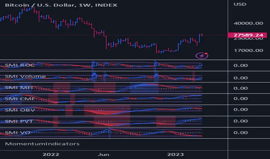
Moving Average Heatmap Visualization7 different types of moving averages (5 different lengths of each) compared to a base moving average. Base moving average can be configured to be a slew of different types of moving averages (credit to @mortdiggiddy for the code) and have a custom length.
Red = base moving average is over other moving average (bearish)
Green = base moving average is under other moving average (bullish)
lengths for the different MAs are just fibonacci numbers due to lack of creativity.
First 5 moving averages are Simple moving average the next 5 are Exponential moving averages and after that it is weighted moving averages, volume weighted moving average (VWAP), Exponential volume weighted moving average (thanks again @mortdiggiddy ), hull moving averages and lastly zero lag moving averages.
The indicator might lag your chart out a bit so be ready for that.
Have fun!
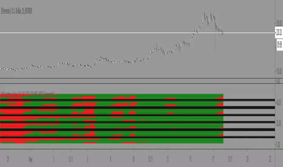
Dskyz (DAFE) MAtrix with ATR-Powered Precision Dskyz (DAFE) MAtrix with ATR-Powered Precision
This cutting‐edge futures trading strategy built to thrive in rapidly changing market conditions. Developed for high-frequency futures trading on instruments such as the CME Mini MNQ, this strategy leverages a matrix of sophisticated moving averages combined with ATR-based filters to pinpoint high-probability entries and exits. Its unique combination of adaptable technical indicators and multi-timeframe trend filtering sets it apart from standard strategies, providing enhanced precision and dynamic responsiveness.
imgur.com
Core Functional Components
1. Advanced Moving Averages
A distinguishing feature of the DAFE strategy is its robust, multi-choice moving averages (MAs). Clients can choose from a wide array of MAs—each with specific strengths—in order to fine-tune their trading signals. The code includes user-defined functions for the following MAs:
imgur.com
Hull Moving Average (HMA):
The hma(src, len) function calculates the HMA by using weighted moving averages (WMAs) to reduce lag considerably while smoothing price data. This function computes an intermediate WMA of half the specified length, then a full-length WMA, and finally applies a further WMA over the square root of the length. This design allows for rapid adaptation to price changes without the typical delays of traditional moving averages.
Triple Exponential Moving Average (TEMA):
Implemented via tema(src, len), TEMA uses three consecutive exponential moving averages (EMAs) to effectively cancel out lag and capture price momentum. The final formula—3 * (ema1 - ema2) + ema3—produces a highly responsive indicator that filters out short-term noise.
Double Exponential Moving Average (DEMA):
Through the dema(src, len) function, DEMA calculates an EMA and then a second EMA on top of it. Its simplified formula of 2 * ema1 - ema2 provides a smoother curve than a single EMA while maintaining enhanced responsiveness.
Volume Weighted Moving Average (VWMA):
With vwma(src, len), this MA accounts for trading volume by weighting the price, thereby offering a more contextual picture of market activity. This is crucial when volume spikes indicate significant moves.
Zero Lag EMA (ZLEMA):
The zlema(src, len) function applies a correction to reduce the inherent lag found in EMAs. By subtracting a calculated lag (based on half the moving average window), ZLEMA is exceptionally attuned to recent price movements.
Arnaud Legoux Moving Average (ALMA):
The alma(src, len, offset, sigma) function introduces ALMA—a type of moving average designed to be less affected by outliers. With parameters for offset and sigma, it allows customization of the degree to which the MA reacts to market noise.
Kaufman Adaptive Moving Average (KAMA):
The custom kama(src, len) function is noteworthy for its adaptive nature. It computes an efficiency ratio by comparing price change against volatility, then dynamically adjusts its smoothing constant. This results in an MA that quickly responds during trending periods while remaining smoothed during consolidation.
Each of these functions—integrated into the strategy—is selectable by the trader (via the fastMAType and slowMAType inputs). This flexibility permits the tailored application of the MA most suited to current market dynamics and individual risk management preferences.
2. ATR-Based Filters and Risk Controls
ATR Calculation and Volatility Filter:
The strategy computes the Average True Range (ATR) over a user-defined period (atrPeriod). ATR is then used to derive both:
Volatility Assessment: Expressed as a ratio of ATR to closing price, ensuring that trades are taken only when volatility remains within a safe, predefined threshold (volatilityThreshold).
ATR-Based Entry Filters: Implemented as atrFilterLong and atrFilterShort, these conditions ensure that for long entries the price is sufficiently above the slow MA and vice versa for shorts. This acts as an additional confirmation filter.
Dynamic Exit Management:
The exit logic employs a dual approach:
Fixed Stop and Profit Target: Stops and targets are set at multiples of ATR (fixedStopMultiplier and profitTargetATRMult), helping manage risk in volatile markets.
Trailing Stop Adjustments: A trailing stop is calculated using the ATR multiplied by a user-defined offset (trailOffset), which captures additional profits as the trade moves favorably while protecting against reversals.
3. Multi-Timeframe Trend Filtering
The strategy enhances its signal reliability by leveraging a secondary, higher timeframe analysis:
15-Minute Trend Analysis:
By retrieving 15-minute moving averages (fastMA15m and slowMA15m) via request.security, the strategy determines the broader market trend. This secondary filter (enabled or disabled through useTrendFilter) ensures that entries are aligned with the prevailing market direction, thereby reducing the incidence of false signals.
4. Signal and Execution Logic
Combined MA Alignment:
The entry conditions are based primarily on the alignment of the fast and slow MAs. A long condition is triggered when the current price is above both MAs and the fast MA is above the slow MA—complemented by the ATR filter and volume conditions. The reverse applies for a short condition.
Volume and Time Window Validation:
Trades are permitted only if the current volume exceeds a minimum (minVolume) and the current hour falls within the predefined trading window (tradingStartHour to tradingEndHour). An additional volume spike check (comparing current volume to a moving average of past volumes) further filters for optimal market conditions.
Comprehensive Order Execution:
The strategy utilizes flexible order execution functions that allow pyramiding (up to 10 positions), ensuring that it can scale into positions as favorable conditions persist. The use of both market entries and automated exits (with profit targets, stop-losses, and trailing stops) ensures that risk is managed at every step.
5. Integrated Dashboard and Metrics
For transparency and real-time analysis, the strategy includes:
On-Chart Visualizations:
Both fast and slow MAs are plotted on the chart, making it easy to see the market’s technical foundation.
Dynamic Metrics Dashboard:
A built-in table displays crucial performance statistics—including current profit/loss, equity, ATR (both raw and as a percentage), and the percentage gap between the moving averages. These metrics offer immediate insight into the health and performance of the strategy.
Input Parameters: Detailed Breakdown
Every input is meticulously designed to offer granular control:
Fast & Slow Lengths:
Determine the window size for the fast and slow moving averages. Smaller values yield more sensitivity, while larger values provide a smoother, delayed response.
Fast/Slow MA Types:
Choose the type of moving average for fast and slow signals. The versatility—from basic SMA and EMA to more complex ones like HMA, TEMA, ZLEMA, ALMA, and KAMA—allows customization to fit different market scenarios.
ATR Parameters:
atrPeriod and atrMultiplier shape the volatility assessment, directly affecting entry filters and risk management through stop-loss and profit target levels.
Trend and Volume Filters:
Inputs such as useTrendFilter, minVolume, and the volume spike condition help confirm that a trade occurs in active, trending markets rather than during periods of low liquidity or market noise.
Trading Hours:
Restricting trade execution to specific hours (tradingStartHour and tradingEndHour) helps avoid illiquid or choppy markets outside of prime trading sessions.
Exit Strategies:
Parameters like trailOffset, profitTargetATRMult, and fixedStopMultiplier provide multiple layers of risk management and profit protection by tailoring how exits are generated relative to current market conditions.
Pyramiding and Fixed Trade Quantity:
The strategy supports multiple entries within a trend (up to 10 positions) and sets a predefined trade quantity (fixedQuantity) to maintain consistent exposure and risk per trade.
Dashboard Controls:
The resetDashboard input allows for on-the-fly resetting of performance metrics, keeping the strategy’s performance dashboard accurate and up-to-date.
Why This Strategy is Truly Exceptional
Multi-Faceted Adaptability:
The ability to switch seamlessly between various moving average types—each suited to particular market conditions—enables the strategy to adapt dynamically. This is a testament to the high level of coding sophistication and market insight infused within the system.
Robust Risk Management:
The integration of ATR-based stops, profit targets, and trailing stops ensures that every trade is executed with well-defined risk parameters. The system is designed to mitigate unexpected market swings while optimizing profit capture.
Comprehensive Market Filtering:
By combining moving average crossovers with volume analysis, volatility thresholds, and multi-timeframe trend filters, the strategy only enters trades under the most favorable conditions. This multi-layered filtering reduces noise and enhances signal quality.
-Final Thoughts-
The Dskyz Adaptive Futures Elite (DAFE) MAtrix with ATR-Powered Precision strategy is not just another trading algorithm—it is a multi-dimensional, fully customizable system built on advanced technical principles and sophisticated risk management techniques. Every function and input parameter has been carefully engineered to provide traders with a system that is both powerful and transparent.
For clients seeking a state-of-the-art trading solution that adapts dynamically to market conditions while maintaining strict discipline in risk management, this strategy truly stands in a class of its own.
****Please show support if you enjoyed this strategy. I'll have more coming out in the near future!!
-Dskyz
Caution
DAFE is experimental, not a profit guarantee. Futures trading risks significant losses due to leverage. Backtest, simulate, and monitor actively before live use. All trading decisions are your responsibility.

Customizable MTF Multiple Moving AveragesTitle:
Customizable Multiple Moving Averages with Dynamic Colors
Description:
This script allows you to calculate up to three customizable moving averages, offering the flexibility to choose from multiple moving average types:
SMA (Simple Moving Average)
EMA (Exponential Moving Average)
WMA (Weighted Moving Average)
VWMA (Volume Weighted Moving Average)
SMMA (Smoothed Moving Average)
Key Features:
Separate Timeframe for Each Moving Average:
Each moving average can be calculated on a different timeframe. For instance, you can display a 1D moving average while working on a 4H chart.
Dynamic Colors:
Moving averages dynamically change color based on their trend:
Uptrend Color: When the moving average is increasing compared to the previous bar of its timeframe.
Downtrend Color: When the moving average is decreasing.
Full Customization:
Length: Adjust the period for each moving average.
Source: Choose any price data source (e.g., close, open, high, low).
Colors: Set custom colors for uptrend and downtrend behavior.
Perfect For:
Multi-Timeframe Trend Analysis:
Observe trends from higher timeframes without switching your current chart.
Crossover Strategies:
Combine multiple moving averages to identify entry and exit signals.
How to Use:
Load the Script: Apply it to your chart.
Configure Inputs: Adjust each moving average's settings from the input panel.
Analyze Trends: Visualize dynamic trend movements with easy-to-identify colors.
Example Configuration:
Set MA1 to a 50-period EMA on a 4H timeframe.
Set MA2 to a 100-period SMMA on a 1D timeframe.
Set MA3 to a 200-period VWMA on a 1W timeframe.
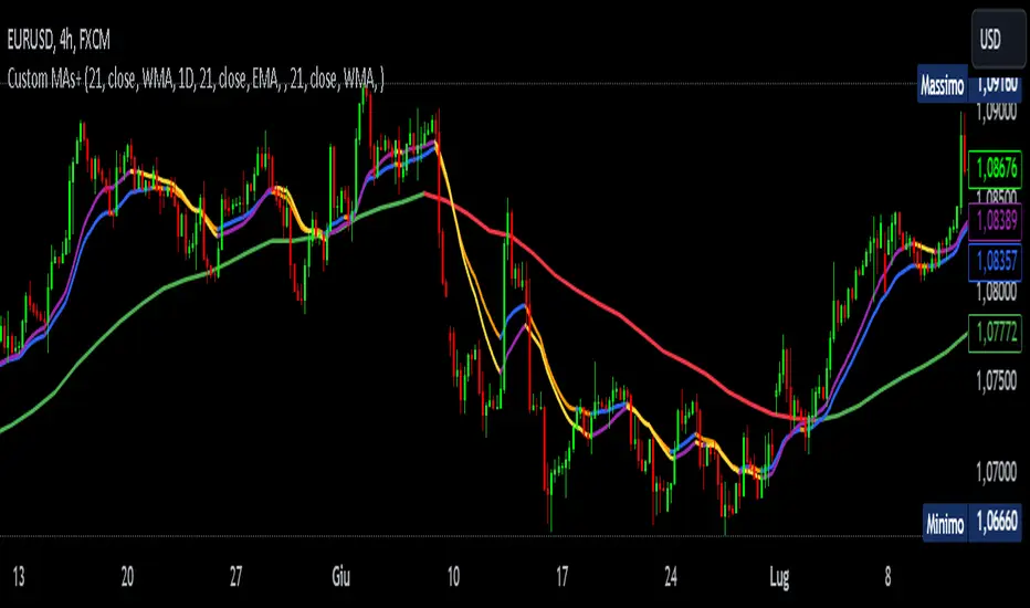
Adaptive DEMA Momentum Oscillator (ADMO)Overview:
The Adaptive DEMA Momentum Oscillator (ADMO) is an open-source technical analysis tool developed to measure market momentum using a Double Exponential Moving Average (DEMA) and adaptive standard deviation. By dynamically combining price deviation from the moving average with normalized standard deviation, ADMO provides traders with a powerful way to interpret market conditions.
Key Features:
Double Exponential Moving Average (DEMA):
The core calculation of the indicator is based on DEMA, which is known for being more responsive to price changes compared to traditional moving averages. This makes the ADMO capable of capturing trend momentum effectively.
Standard Deviation Integration:
A normalized standard deviation is used to adaptively weight the oscillator. This makes the indicator more sensitive to market volatility, enhancing responsiveness during high volatility and reducing sensitivity during calmer periods.
Oscillator Representation:
The final oscillator value is derived from the combination of the DEMA-based Z-score and the normalized standard deviation. This final value is visualized as a color-coded histogram, reflecting bullish or bearish momentum.
Color-Coded Histogram:
Bullish Momentum: Values above zero are colored using a customizable bullish color (default: light green).
Bearish Momentum: Values below zero are colored using a customizable bearish color (default: red).
How It Works:
Inputs:
DEMA Length: Defines the period used for calculating the Double Exponential Moving Average. It can be adjusted from 1 to 200 to suit different trading styles.
Standard Deviation Length: Sets the lookback period for standard deviation calculations, which influences the responsiveness of the oscillator.
Standard Deviation Weight (StdDev Weight): Controls the weight given to the normalized standard deviation, allowing customization of the oscillator's sensitivity to volatility.
Calculation Steps:
Double Exponential Moving Average Calculation:
The DEMA is calculated using two exponential moving averages, which helps in reducing lag compared to a simple moving average.
Z-score Calculation:
The Z-score is derived by comparing the difference between the DEMA and its smoothed average (LSMA) to the standard deviation. This indicates how far the current value is from the mean in units of standard deviation.
Normalized Standard Deviation:
The standard deviation is normalized by subtracting the mean standard deviation and dividing by the standard deviation of the values. This helps to make the oscillator adaptive to recent changes in volatility.
Final Oscillator Value:
The final value is calculated by multiplying the Z-score with a factor based on the normalized standard deviation, resulting in a momentum indicator that adapts to different market conditions.
Visualization:
Histogram: The oscillator is plotted as a histogram, with color-coded bars showing the strength and direction of market momentum.
Positive (bullish) values are shown in green, indicating upward momentum.
Negative (bearish) values are shown in red, indicating downward momentum.
Zero Line: A zero line is plotted to provide a reference point, helping users quickly determine whether the current momentum is bullish or bearish.
Example Use Cases:
Momentum Identification:
ADMO helps identify the current market momentum by dynamically adapting to changes in market volatility. When the histogram is above zero and green, it indicates bullish conditions, whereas values below zero and red suggest bearish momentum.
Volatility-Adjusted Signals:
The normalized standard deviation weighting allows the ADMO to provide more reliable signals during different market conditions. This makes it particularly useful for traders who want to be responsive to market volatility while avoiding false signals.
Trend Confirmation and Divergence:
ADMO can be used to confirm the strength of a trend or identify potential divergences between price and momentum. This helps traders spot potential reversal points or continuation signals.
Summary:
The Adaptive DEMA Momentum Oscillator (ADMO) offers a unique approach by combining momentum analysis with adaptive standard deviation. The integration of DEMA makes it responsive to price changes, while the standard deviation adjustment helps it stay relevant in both high and low volatility environments. It's a versatile tool for traders who need an adaptive, momentum-based approach to technical analysis.
Feel free to explore the code and adapt it to your trading strategy. The open-source nature of this tool allows you to adjust the settings and visualize the output to fit your personal trading preferences.

Quarterly Sine Wave with Moving Averages - AYNETDescription
Sine Wave:
The sine wave oscillates with a frequency determined by frequency.
Its amplitude (amplitude) and vertical offset (offset) are adjustable.
Moving Averages:
Includes options for different types of moving averages:
SMA (Simple Moving Average).
EMA (Exponential Moving Average).
WMA (Weighted Moving Average).
HMA (Hull Moving Average).
The user can choose the type (ma_type) and the length (ma_length) via inputs.
Horizontal Lines:
highest_hype and lowest_hype are horizontal levels drawn at the user-specified values.
Quarter Markers:
Vertical lines and labels (Q1, Q2, etc.) are drawn at the start of each quarter.
Customization Options
Moving Average Type:
Switch between SMA, EMA, WMA, and HMA using the dropdown menu.
Sine Wave Frequency:
Adjust the number of oscillations per year.
Amplitude and Offset:
Control the height and center position of the sine wave.
Moving Average Length:
Change the length for any selected moving average.
Output
This indicator plots:
A sine wave that oscillates smoothly over the year, divided into quarters.
A customizable moving average calculated based on the chosen price (e.g., close).
Horizontal lines for the highest and lowest hype levels.
Vertical lines and labels marking the start of each quarter.
Let me know if you need additional features! 😊
